Project description
Samples
naïve_KO3 (SRR26891264): SRR26891264naïve_KO2 (SRR26891265): SRR26891265
naïve_KO1 (SRR26891266): SRR26891266
naïve_WT3 (SRR26891267): SRR26891267
naïve_WT2 (SRR26891268): SRR26891268
naïve_WT1 (SRR26891269): SRR26891269
Making project directories
mkdir -p /data/rnaseq/{index_mouse,PRJNA1043092/{rawdata,QC,trim_data,bam,count_matrix}}
Setting variables
GTF=/data/rnaseq/mouse_GFT39/Mus_musculus.GRCm39.113.gtf
genome=/data/rnaseq/mouse_genome39/Mus_musculus.GRCm39.dna.primary_assembly.fa
index=/data/rnaseq/index_mouse
reads=/data/rnaseq/PRJNA1043092/rawdata
qc=/data/rnaseq/PRJNA1043092/QC
trim=/data/rnaseq/PRJNA1043092/trim_data
bam=/data/rnaseq/PRJNA1043092/bam
count=/data/rnaseq/PRJNA1043092/count_matrix
Downloading raw data
The tsv file was downloaded from: PRJNA1043092 and was renamed to bulk_RNA_seq.txt.Making list of ftp addresses for each sample, and list of new sample names
list_of_samples=(SRR26891264 SRR26891265 SRR26891266 SRR26891267 SRR26891268 SRR26891269)
for i in $list_of_samples; do grep $i bulk_RNA_seq.txt | awk '{print $8}' | awk '{gsub(/\;/,"\n")};{print $0}'>>samples.sh;done
for sample in $list_of_samples;do echo wget -O ${reads}/${sample}_1.fastq.gz>>names.sh; echo wget -O ${reads}/${sample}_2.fastq.gz>>names.sh;done
paste -d " " names.sh samples.sh>download.sh
bash download.sh
wget -O /data/rnaseq/PRJNA1043092/rawdata/SRR26891264_1.fastq.gz ftp.sra.ebi.ac.uk/vol1/fastq/SRR268/064/SRR26891264/SRR26891264_1.fastq.gz
wget -O /data/rnaseq/PRJNA1043092/rawdata/SRR26891264_2.fastq.gz ftp.sra.ebi.ac.uk/vol1/fastq/SRR268/064/SRR26891264/SRR26891264_2.fastq.gz
wget -O /data/rnaseq/PRJNA1043092/rawdata/SRR26891265_1.fastq.gz ftp.sra.ebi.ac.uk/vol1/fastq/SRR268/065/SRR26891265/SRR26891265_1.fastq.gz
wget -O /data/rnaseq/PRJNA1043092/rawdata/SRR26891265_2.fastq.gz ftp.sra.ebi.ac.uk/vol1/fastq/SRR268/065/SRR26891265/SRR26891265_2.fastq.gz
wget -O /data/rnaseq/PRJNA1043092/rawdata/SRR26891266_1.fastq.gz ftp.sra.ebi.ac.uk/vol1/fastq/SRR268/066/SRR26891266/SRR26891266_1.fastq.gz
wget -O /data/rnaseq/PRJNA1043092/rawdata/SRR26891266_2.fastq.gz ftp.sra.ebi.ac.uk/vol1/fastq/SRR268/066/SRR26891266/SRR26891266_2.fastq.gz
wget -O /data/rnaseq/PRJNA1043092/rawdata/SRR26891267_1.fastq.gz ftp.sra.ebi.ac.uk/vol1/fastq/SRR268/067/SRR26891267/SRR26891267_1.fastq.gz
wget -O /data/rnaseq/PRJNA1043092/rawdata/SRR26891267_2.fastq.gz ftp.sra.ebi.ac.uk/vol1/fastq/SRR268/067/SRR26891267/SRR26891267_2.fastq.gz
wget -O /data/rnaseq/PRJNA1043092/rawdata/SRR26891268_1.fastq.gz ftp.sra.ebi.ac.uk/vol1/fastq/SRR268/068/SRR26891268/SRR26891268_1.fastq.gz
wget -O /data/rnaseq/PRJNA1043092/rawdata/SRR26891268_2.fastq.gz ftp.sra.ebi.ac.uk/vol1/fastq/SRR268/068/SRR26891268/SRR26891268_2.fastq.gz
wget -O /data/rnaseq/PRJNA1043092/rawdata/SRR26891269_1.fastq.gz ftp.sra.ebi.ac.uk/vol1/fastq/SRR268/069/SRR26891269/SRR26891269_1.fastq.gz
wget -O /data/rnaseq/PRJNA1043092/rawdata/SRR26891269_2.fastq.gz ftp.sra.ebi.ac.uk/vol1/fastq/SRR268/069/SRR26891269/SRR26891269_2.fastq.gz
Building STAR (Spliced Transcripts Alignment to a Reference) index
STAR --runThreadN 4 \
--runMode genomeGenerate \
--genomeDir $index \
--genomeFastaFiles $genome \
--sjdbGTFfile $GTF \
--sjdbOverhang 149
Quality control
for sample in $reads/*.fastq.gz; do
fastqc $sample -o ${qc}/
done
Before trimming
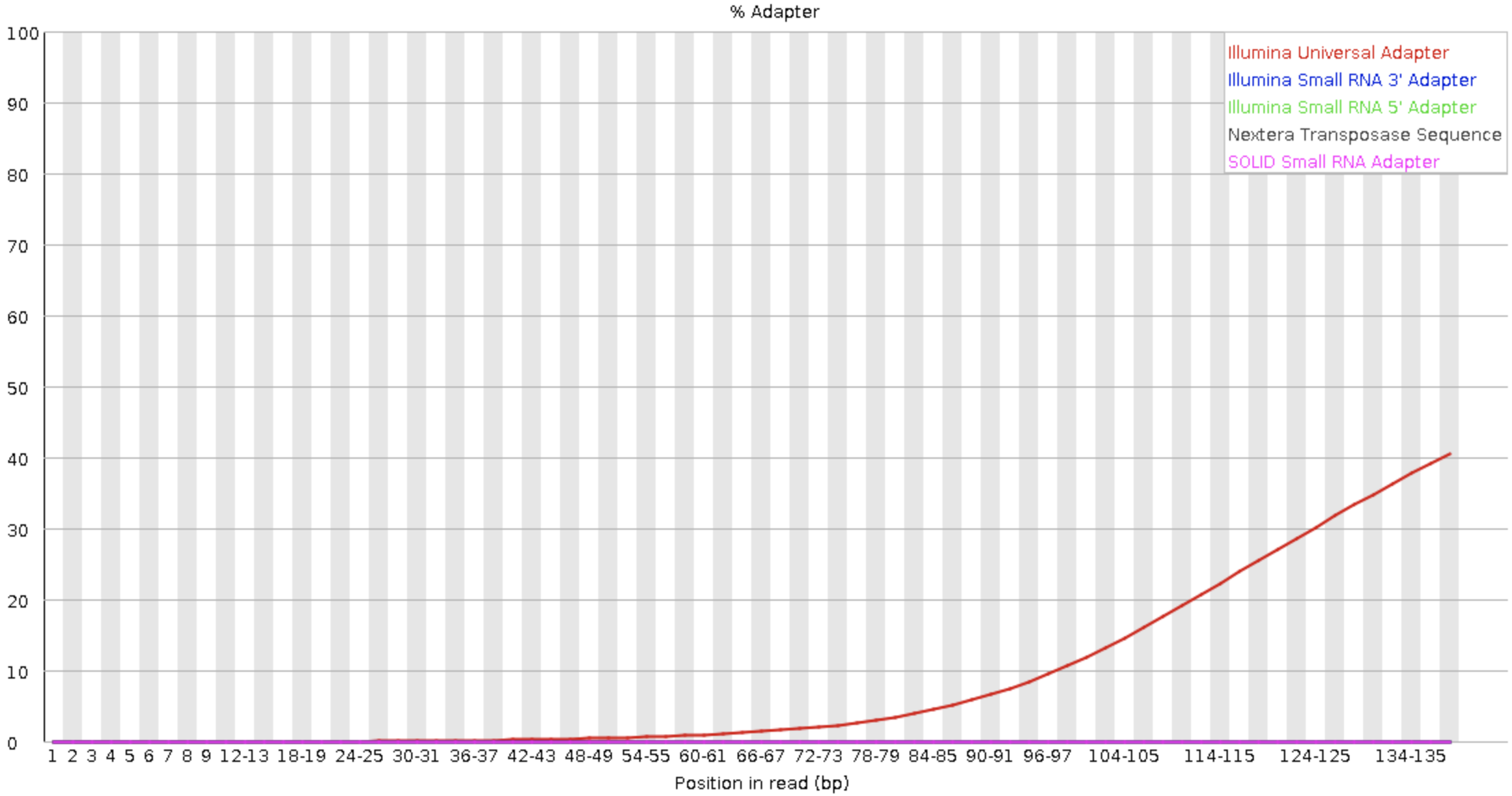
Removing adapters and low quality bases
for base in SRR26891264 SRR26891265 SRR26891266 SRR26891267 SRR26891268 SRR26891269
do
fq1=$reads/${base}_1.fastq.gz
fq2=$reads/${base}_2.fastq.gz

cutadapt -q 20 -O 9 -m 45 -a AGATCGGAAGAGCACACGTCTGAACTCCAGTCA -A AGATCGGAAGAGCGTCGTGTAGGGAAAGAGTGT -o $trim/${base}_trim_1.fastq.gz -p $trim/${base}_trim_2.fastq.gz $fq1 $fq2
done
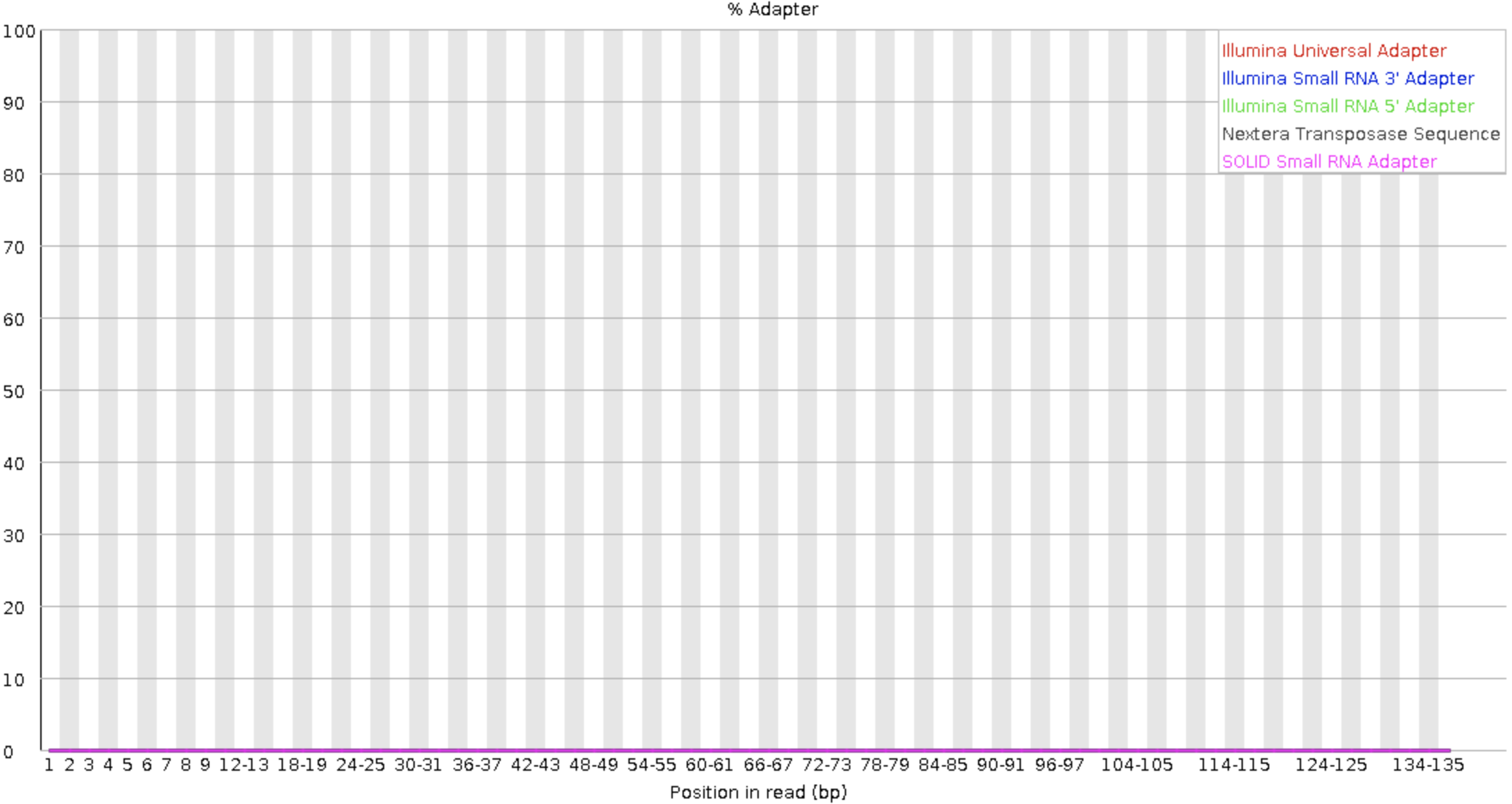
Quality control of trimmed data
for sample in $trim/*.fastq.gz
do
fastqc $sample -o ${qc}
done
After trimming
Reads alignment
for base in SRR26891264 SRR26891265 SRR26891266 SRR26891267 SRR26891268 SRR26891269
do
fq1=$trim/${base}_trim_1.fastq.gz
fq2=$trim/${base}_trim_2.fastq.gz

# align with STAR (Spliced Transcripts Alignment to a Reference)
STAR --runThreadN 32 --genomeDir $index --readFilesIn $fq1 $fq2 --outSAMtype BAM Unsorted --quantMode GeneCounts --readFilesCommand zcat --outFileNamePrefix $trim/$base
done
Count matrix
With STAR option --quantMode GeneCounts output of STAR contains count matrix sample_nameReadsPerGene.out.tab. That count matrix contains 4 columns which correspond to different strandedness options:column 1: gene ID
column 2: counts for unstranded RNA-seq
column 3: counts for the 1st read strand aligned with RNA (htseq-count option -s yes, featureCounts option -s -1)
column 4: counts for the 2nd read strand aligned with RNA (htseq-count option -s reverse, featureCounts option -s -2)
Checking if RNA-seq protocol is stranded
grep -v "N_" ${trim}/SRR26891264ReadsPerGene.out.tab | awk '{unst+=$2;forw+=$3;rev+=$4}END{print unst,forw,rev}'
18769322 2598512 18432547
Concatenating all count matrix files into one text file
list=${trim}/SRR26891269,${trim}/SRR26891268,${trim}/SRR26891267,${trim}/SRR26891266,${trim}/SRR26891265,${trim}/SRR26891264
grep -v "N_" ${trim}/SRR26891264ReadsPerGene.out.tab | awk '{print $1}' >countMatrix.txt
for file in $(echo ${list} | tr "," " "); do
        grep -v "N_" ${file}ReadsPerGene.out.tab | cut -f4 | paste -d " " countMatrix.txt - > temp.txt
        mv temp.txt countMatrix.txt
done
Analysis in R
raw_count<-read.table("/Users/alexeyefanov/Desktop/Programming/rnaseq_analysis/Palmisano_rnaseq/count_matrix/countMatrix.txt", sep=" ")
colnames(raw_count)<-c("ID", "WT1", "WT2", "WT3", "KO1", "KO2", "KO3")
head(raw_count)
A data.frame: 6 × 7
                  ID WT1 WT2 WT3 KO1 KO2 KO3

1 ENSMUSG00000104478   0   0   0   1   0   0
2 ENSMUSG00000104385   3   1   0   1   0   2
3 ENSMUSG00000101231   0   0   0   0   0   0
4 ENSMUSG00000102135   1   0   0   0   1   0
5 ENSMUSG00000103282   0   0   0   0   0   0
6 ENSMUSG00000101097   0   0   0   0   0   0
rownames(raw_count)<-raw_count$ID
raw_count$ID<-NULL
sample<-c("WT1","WT2","WT3","KO1","KO2","KO3")
condition<-c("control","control","control","experiment","experiment","experiment")
metadata<-data.frame(sample, condition)
head(metadata)
A data.frame: 6 × 2
sample  condition

1 WT1   control
2 WT2   control
3 WT3   control
4 KO1   experiment
5 KO2   experiment
6 KO3   experiment
rownames(metadata)<-metadata$sample
metadata$sample<-NULL
which(is.na(raw_count$WT1))
which(is.na(raw_count$WT2))
which(is.na(raw_count$WT3))
which(is.na(raw_count$KO1))
which(is.na(raw_count$KO2))
which(is.na(raw_count$KO3))
all(rownames(metadata)==colnames(raw_count))
TRUE
keep<-rowSums(raw_count)>10
raw_count_deseq_cleaned<-raw_count[keep,]
nrow(raw_count_deseq_cleaned)
31298
raw_count_deseq_cleaned$entrez<-mapIds(org.Mm.eg.db, key=rownames(raw_count_deseq_cleaned), keytype="ENSEMBL", column="SYMBOL")
raw_count_deseq_cleaned<-raw_count_deseq_cleaned[!duplicated(raw_count_deseq_cleaned$entrez), ]
raw_count_deseq_cleaned<-na.omit(raw_count_deseq_cleaned)
rownames(raw_count_deseq_cleaned)<-raw_count_deseq_cleaned$entrez
raw_count_deseq_cleaned$entrez<-NULL
dim(raw_count_deseq_cleaned)
18947 7
Downstream analysis was performed in Bioconductor (DESeq2, clusterProfiler)
Making the DESeqDataSet object
dds<-DESeqDataSetFromMatrix(countData=raw_count_deseq_cleaned, colData=metadata, design=~condition)
dds<-estimateSizeFactors(dds)
sizeFactors(dds)
WT1 1.27432842508796 WT2 1.06065569907931 WT3 0.830457939984845

KO1 1.18880822849783 KO2 0.875296687050556 KO3 0.878336725432078
vst_tr<-vst(dds, blind=TRUE)
library(repr)
library(ggplot2)
options(repr.plot.width=7, repr.plot.height=4)
pca<-plotPCA(vst_tr)+ggtitle("PCA plot")+theme(plot.title=element_text(size=16, hjust=0.5))+
geom_text(aes(label = colnames(vst_tr)), hjust =-0.2, vjust = -0.2)+xlim(-13,14)
pca
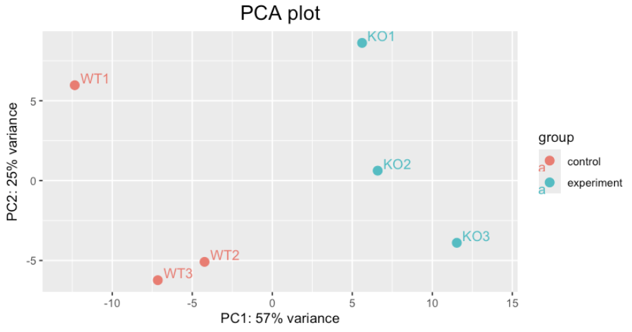 The WT1 sample might be an outlier.
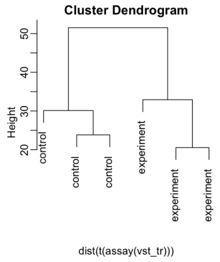
Making cluster dendrogram
t(assay(vst_tr))
mypar(1,2)
den<-plot(hclust(dist(t(assay(vst_tr)))), labels=colData(dds)$condition)
den
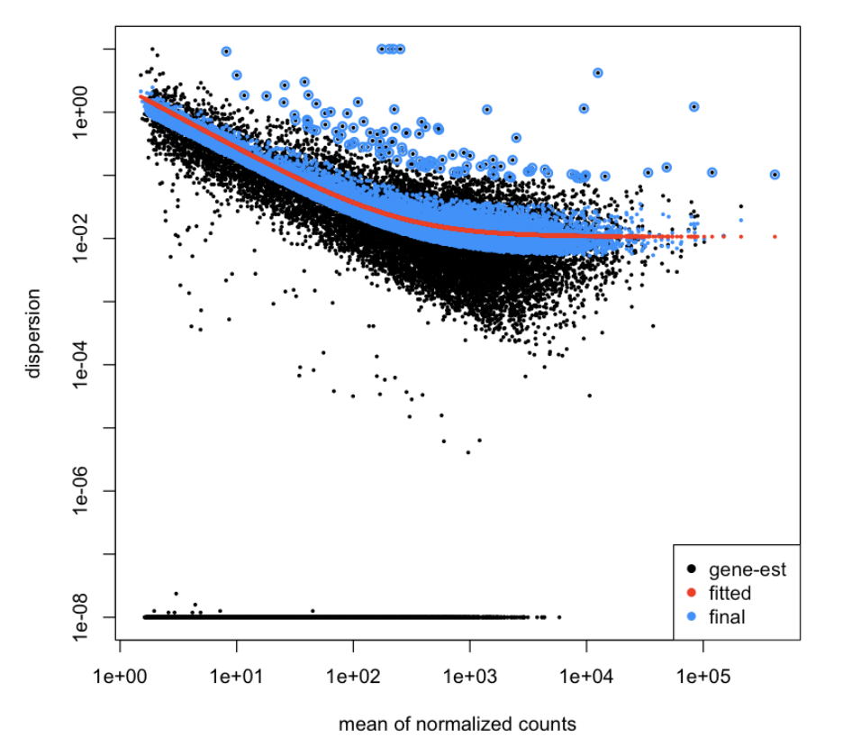
Building a model and plotting a graph displaying dispersion vs mean of normalized counts
dds<-DESeq(dds)
plotDispEsts(dds)
Making dataframe containing DE genes
results<-results(dds, contrast=c("condition", "experiment", "control"), alpha=0.05)
head(results, 3)
log2 fold change (MLE): condition experiment vs control
Wald test p-value: condition experiment vs control
DataFrame with 3 rows and 6 columns
        baseMean log2FoldChange     lfcSE      stat    pvalue      padj

Gm8141   12.4239       0.355419  0.556622  0.638528  0.523130  0.835953
Pcmtd1 1149.8843       0.138119  0.129156  1.069396  0.284891  0.685673
Cdh7     64.6494       0.165669  0.264059  0.627394  0.530401  0.840182
summary(results)
out of 18946 with nonzero total read count
adjusted p-value < 0.05
LFC > 0 (up)       : 212, 1.1%
LFC < 0 (down)     : 709, 3.7%
outliers [1]       : 7, 0.037%
low counts [2]     : 2572, 14%
(mean count < 7)
[1] see 'cooksCutoff' argument of ?results
[2] see 'independentFiltering' argument of ?results
DESeq2::plotMA(results, ylim=c(-4,4))
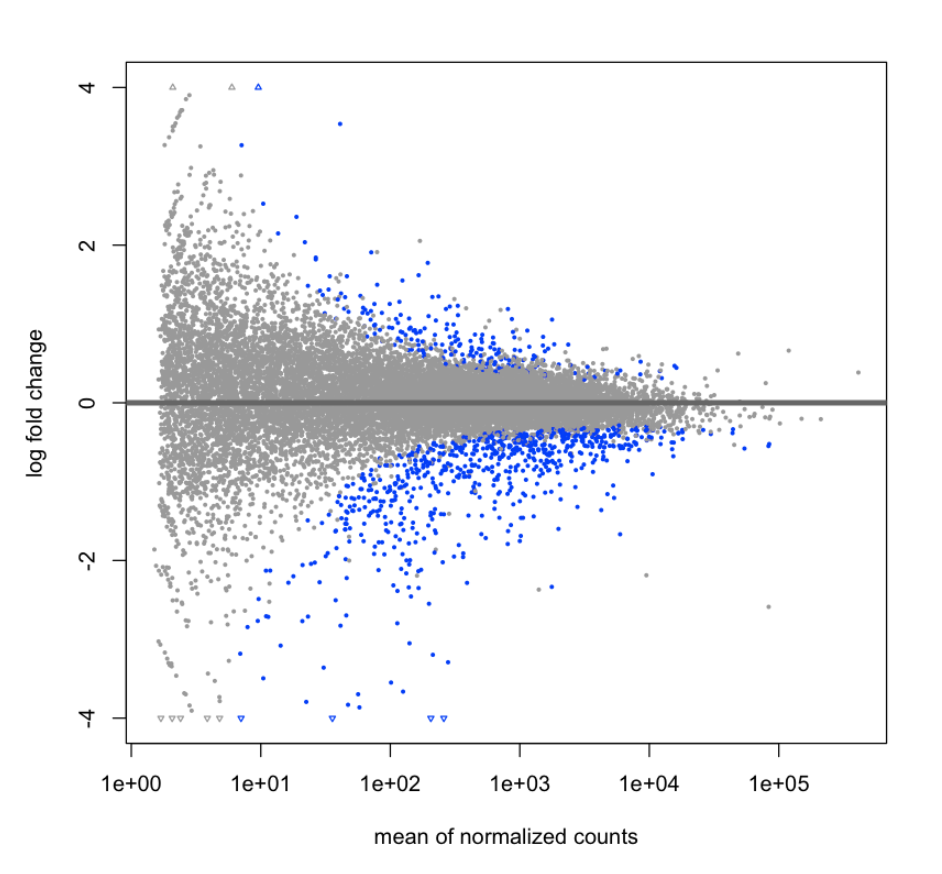
results<-subset(results, padj<0.05)
nrow(results)
921
Gene ontology and functional testing
Next, we extract all genes which are included in the TxDb object to use as our universe of genes for pathway enrichment.
allGeneGR <- genes(TxDb.Mmusculus.UCSC.mm39.knownGene)
allGeneIDs <- allGeneGR$gene_id
results<-results[order(results$log2FoldChange, decreasing=TRUE),]
results$gene_id<-mapIds(org.Mm.eg.db, key=rownames(results), keytype="SYMBOL", column="ENTREZID")
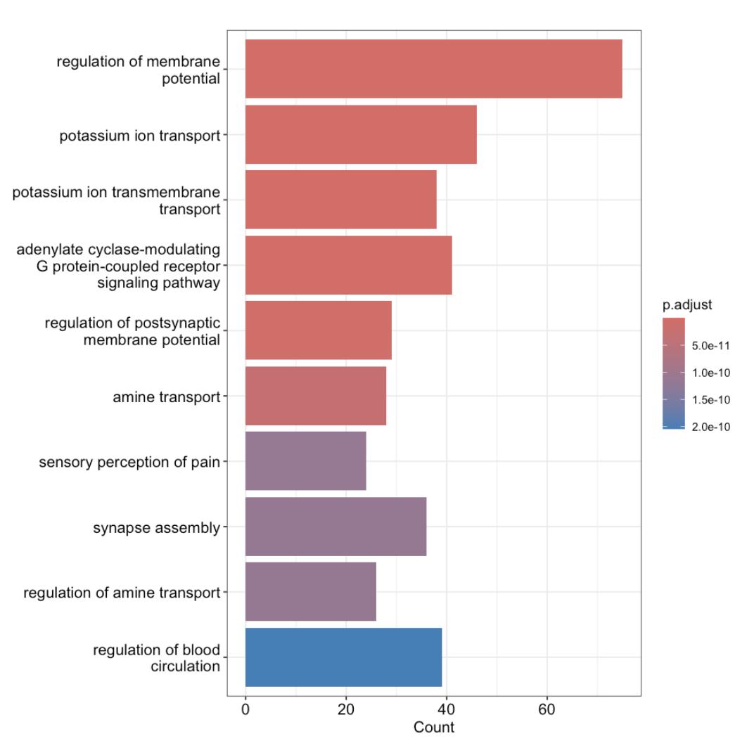
GO_result <- enrichGO(gene = results$gene_id, universe = allGeneIDs, OrgDb = org.Mm.eg.db,
    ont = "BP")
barplot(GO_result, showCategory = 10)
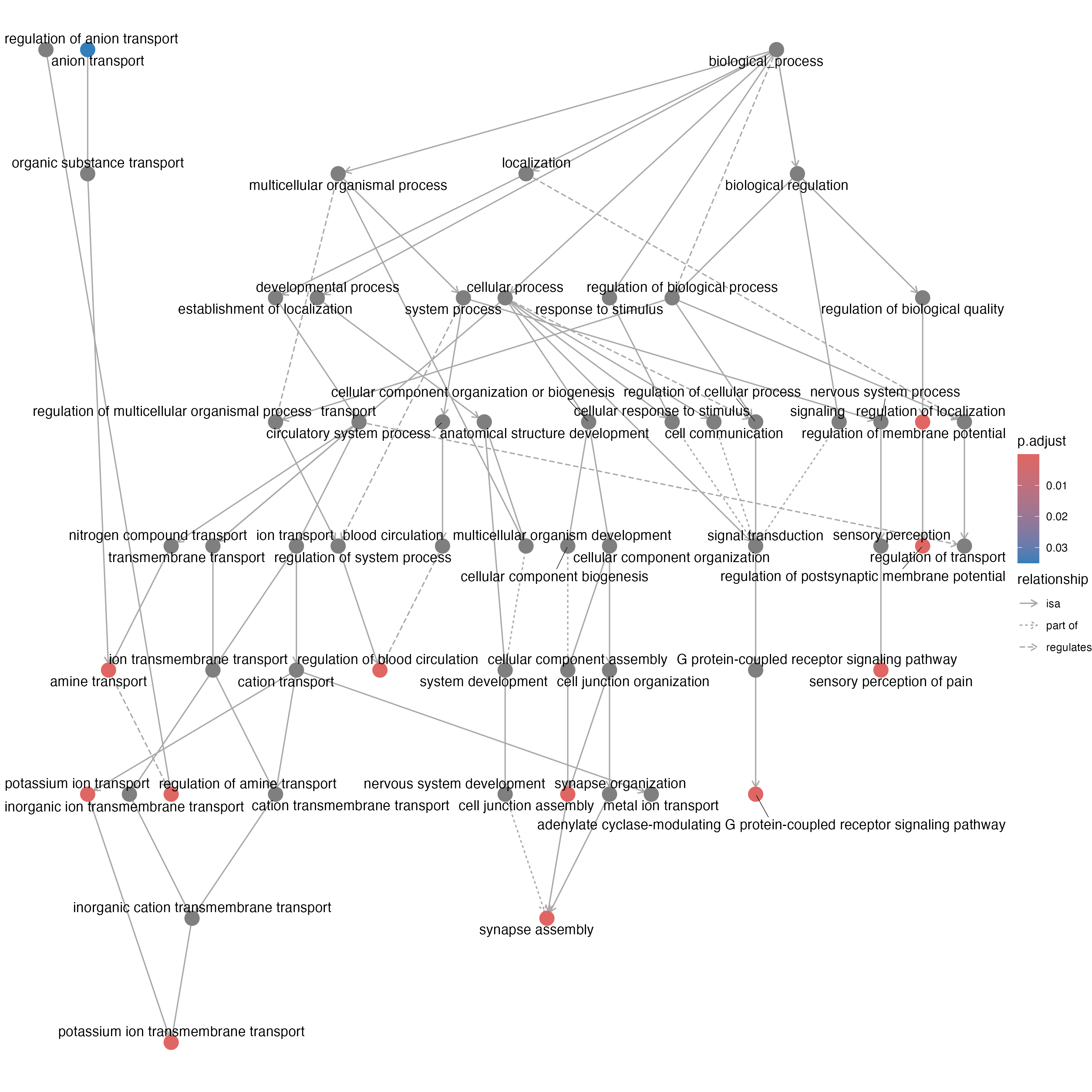
Visualize enriched GO terms as a directed acyclic graph
options(repr.plot.width=20, repr.plot.height=15)
p<-goplot(GO_result)
ggsave(p, file="/Users/alexeyefanov/test_site/mysite/bioinformatics/images/graph.png", width = 12, height = 12)
Conclusion
- Totally, 921 DE genes were detected in the current study.
- 212 DE genes were upregulated and 709 were downregulated
- Several GO terms were enriched in KO mice vs WT mice including:potassium ion transport, adenylate cyclase- modulating G protein-coupled receptor signaling pathway, and synapse assembly
Back to bioinformatics project page: Back to bioinformatics project page
Back to home: Back to home