Project description
Link to myc Chip-seq data: myc
Link to control Chip-seq data: control
Raw data downloding and reads mapping
Raw data were downloaded by the following commands:
wget https://www.encodeproject.org/files/ENCFF001NQP/@@download/ENCFF001NQP.fastq.gz
wget https://www.encodeproject.org/files/ENCFF001NQQ/@@download/ENCFF001NQQ.fastq.gz
wget https://www.encodeproject.org/files/ENCFF001NCH/@@download/ENCFF001NCH.fastq.gz
wget https://www.encodeproject.org/files/ENCFF001NCF/@@download/ENCFF001NCF.fastq.gz
mv ENCFF001NQP.fastq.gz rep1.fastq.gz
mv ENCFF001NQQ.fastq.gz rep2.fastq.gz
mv ENCFF001NCH.fastq.gz input1.fastq.gz
mv ENCFF001NCF.fastq.gz input2.fastq.gz
fqSample <- FastqSampler("/Users/alexeyefanov/Desktop/Programming/Bioconductor/ChiP-seq/MEL/data/raw_data/rep1.fastq.gz", n = 10^6)
fastq <- yield(fqSample)
fastq
class: ShortReadQ
length: 1000000 reads; width: 36 cycles
Raw ChIPseq data QC
We can access different metrics of fastq files by following functions:sread() - Retrieve sequence of reads.
quality() - Retrieve quality of reads as ASCII scores.
id() - Retrieve IDs of reads.
readSequences <- sread(fastq)
readQuality <- quality(fastq)
readIDs <- id(fastq)
readSequences
DNAStringSet object of length 1000000:
          width seq
      [1]    36 ACAGTAGTCTTCCGGTCAAGAGCTACACGGGTTGTG
      [2]    36 TGTGTGTATGTCTGCCTGCCAGCAGAGGGAACCAGA
      [3]    36 CTGATTCAAACTCTGTTCTGTCAGCTTCTGACTGAA
      [4]    36 AGATACCATATAATGAACCCACGAAAACAATCCGGT
      [5]    36 CTAAAATAACCAAAGGACTTGTCACATCTATGTAAA
      ...   ... ...
 [999996]    36 GTTTATAAACAGCATTGTACGTTACCCAGGACCTGC
 [999997]    36 AAACAGGAGGAAGGGAGGATTGAGGGACCGCACAGA
 [999998]    36 CAACAGGTTTGATCTTCACGCTCGGCTTATTCTTGC
 [999999]    36 GTGACTTTACCCGCTTTATCTCTGGACTCCAGAGTT
[1000000]    36 TTTCCTACTTTACAGCATAGATGATGAAAAACACAA
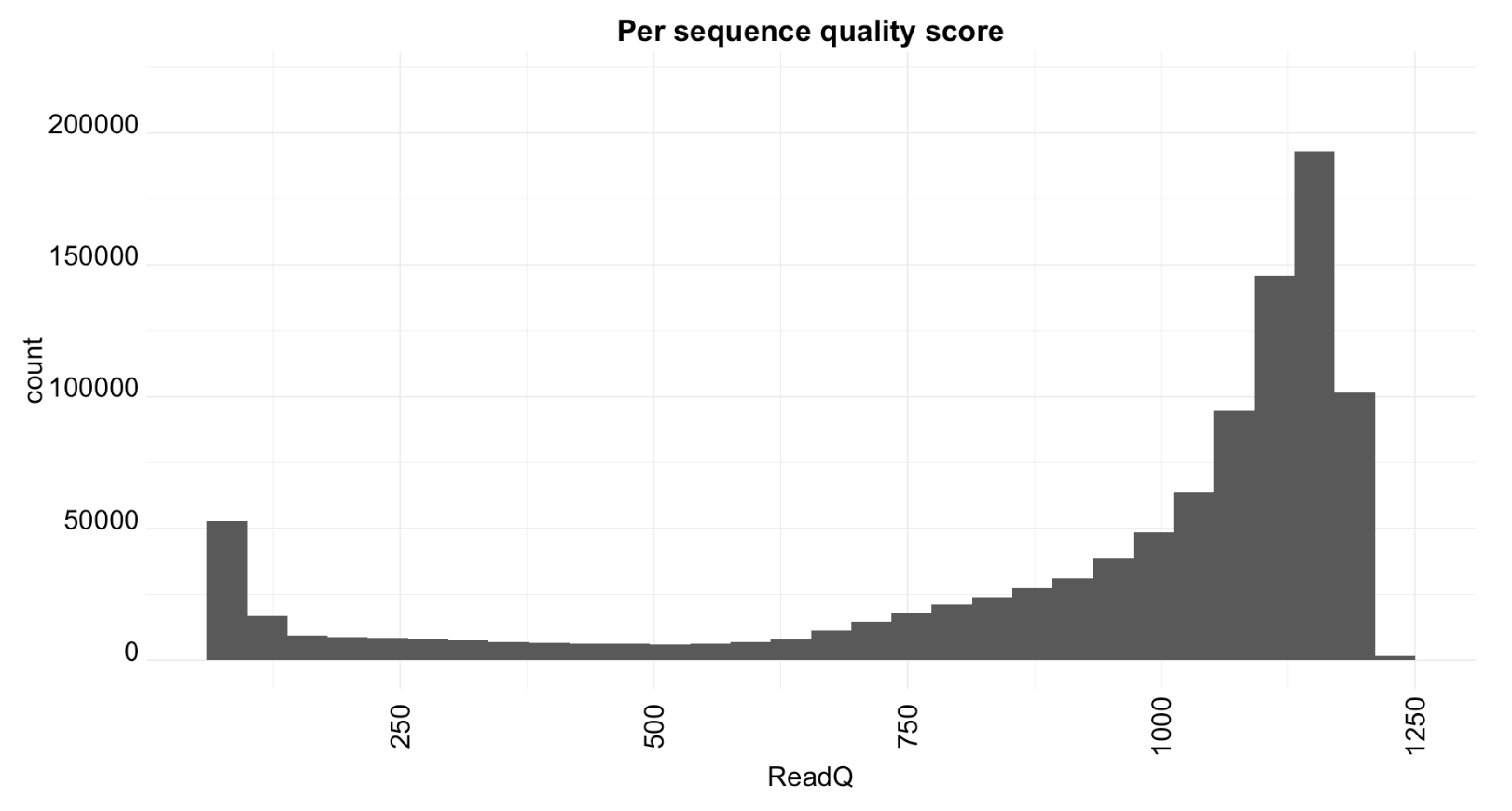
Histogram of quality scores.
library(ggplot2)
library(repr)
options(repr.plot.width=15, repr.plot.height=8)
toPlot <- data.frame(ReadQ = readQualities)
ggplot(toPlot, aes(x = ReadQ)) + geom_histogram(bins=30) + theme_minimal()+
theme(axis.text.x = element_text(color = "black", size = 20, angle = 90, hjust = .5, vjust = .5, face = "plain"),
        axis.text.y = element_text(color = "black", size = 20, angle = 0, hjust = 1, vjust = 0, face = "plain"),
        axis.title.x = element_text(color = "black", size = 20, angle = 0, hjust = .5, vjust = 0, face = "plain"),
        axis.title.y = element_text(color = "black", size = 20, angle = 90, hjust = .5, vjust = .5, face = "plain"),
     plot.title = element_text(size=22, hjust = .5, vjust = .5, face="bold"))+
ylim(0, 220000)+ggtitle("Per sequence quality score")
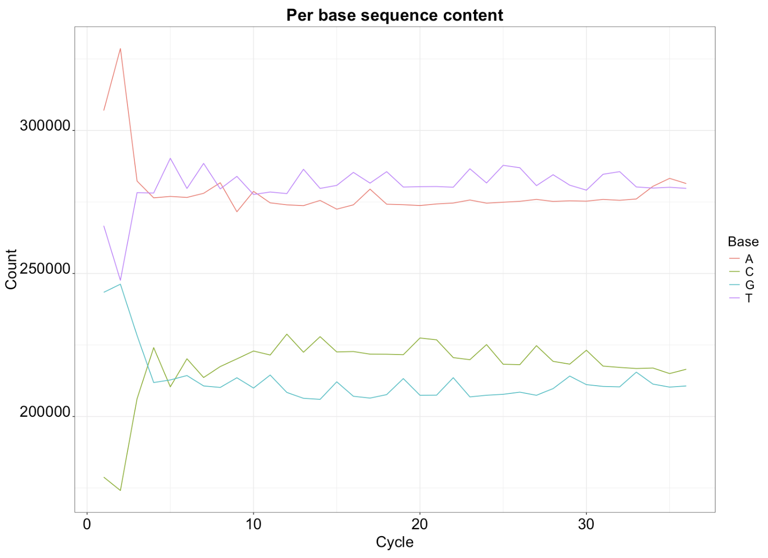
Visualizing base occurrence over positions in reads
readSequences_AlpbyCycle <- alphabetByCycle(readSequences)
readSequences_AlpbyCycle[1:4, 1:10]
                             A matrix: 4 × 10 of type int
A 306954  328614  282305  276432  276920  276570  278020  281716  271557  278703
C 178805  174129  206175  224071  210374  220172  213623  217461  220140  222889
G 243413  246240  228349  211866  212787  214306  210685  210163  213540  209952
T 266665  247611  278246  278121  290270  279718  288472  279555  283949  277603
AFreq <- readSequences_AlpbyCycle["A", ]
CFreq <- readSequences_AlpbyCycle["C", ]
GFreq <- readSequences_AlpbyCycle["G", ]
TFreq <- readSequences_AlpbyCycle["T", ]
toPlot <- data.frame(Count = c(AFreq, CFreq, GFreq, TFreq), Cycle = rep(1:36, 4),
    Base = rep(c("A", "C", "G", "T"), each = 36))
ggplot(toPlot, aes(y = Count, x = Cycle, colour = Base)) + geom_line() + theme_bw()+
theme(axis.text.x = element_text(color = "black", size = 20, angle =0, hjust = .5, vjust = .5, face = "plain"),
        axis.text.y = element_text(color = "black", size = 20, angle = 0, hjust = 1, vjust = 0, face = "plain"),
        axis.title.x = element_text(color = "black", size = 20, angle = 0, hjust = .5, vjust = 0, face = "plain"),
        axis.title.y = element_text(color = "black", size = 20, angle = 90, hjust = .5, vjust = .5, face = "plain"),
     plot.title = element_text(size=22, hjust = .5, vjust = .5, face="bold"))+
  theme(
    legend.text = element_text(size = 16),
    legend.title = element_text(size = 18))+ggtitle("Per base sequence content")
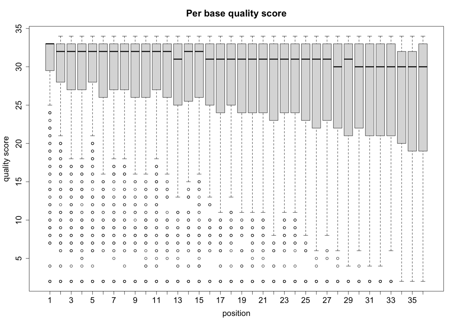
Per base quality score
options(repr.plot.width=14, repr.plot.height=10)
graphics::boxplot(qualAsMatrix[1:1000, ], xlab="position", ylab="quality score", main="Per base quality score", cex.axis=1.5, cex.lab=1.5, cex.main=1.75)
Filtering out the low quality reads
Low quality reads will be filtered out based on following criteria:Quality score more than 300
The number of N in the read is less than 10
First, path to filterd reads was created:
files <- list.files(path="/Users/alexeyefanov/Desktop/Programming/Bioconductor/ChiP-seq/MEL/data",pattern="*.fastq.gz")
files_filt<- paste("filt", files, sep = "_")
path_filt<-paste0("/Users/alexeyefanov/Desktop/Programming/Bioconductor/ChiP-seq/MEL/data/", files_filt)
path_filt
'/Users/alexeyefanov/Desktop/Programming/Bioconductor/ChiP-seq/MEL/data/filt_input1.fastq.gz'
'/Users/alexeyefanov/Desktop/Programming/Bioconductor/ChiP-seq/MEL/data/filt_input2.fastq.gz'
'/Users/alexeyefanov/Desktop/Programming/Bioconductor/ChiP-seq/MEL/data/filt_rep1.fastq.gz'
'/Users/alexeyefanov/Desktop/Programming/Bioconductor/ChiP-seq/MEL/data/filt_rep2.fastq.gz'
mylist <- lapply(paste0("/Users/alexeyefanov/Desktop/Programming/Bioconductor/ChiP-seq/MEL/data/",files), function(x) FastqStreamer(x, n = 1e+05))
mylist
[[1]]
class: FastqStreamer
file: input1.fastq.gz
status: n=100000 current=0 added=0 total=0 buffer=0

[[2]]
class: FastqStreamer
file: input2.fastq.gz
status: n=100000 current=0 added=0 total=0 buffer=0

[[3]]
class: FastqStreamer
file: rep1.fastq.gz
status: n=100000 current=0 added=0 total=0 buffer=0

[[4]]
class: FastqStreamer
file: rep2.fastq.gz
status: n=100000 current=0 added=0 total=0 buffer=0
k=1
for (i in mylist){
TotalReads <- 0
TotalReadsFilt <- 0

while (length(fq <- yield(i)) > 0) {
    TotalReads <- TotalReads + length(fq)
    filt1 <- fq[alphabetScore(fq) > 300]
    filt2 <- filt1[alphabetFrequency(sread(filt1))[, "N"] < 10]
    TotalReadsFilt <- TotalReadsFilt + length(filt2)
    writeFastq(filt2, path_filt[k], mode = "a")
    k=k+1
}
}
Reads mapping and peaks calling
Reads mapping and peaks calling were performed in zsh shell.bowtie2 was used for reads mapping
macs2 was used for peak calling
index=/Users/alexeyefanov/Desktop/Programming/Bioconductor/refgenomes/mouse_index
filt=/Users/alexeyefanov/Desktop/Programming/Bioconductor/ChiP-seq/MEL/data/filtered
reference=/Users/alexeyefanov/Desktop/Programming/Bioconductor/refgenomes/BSgenome.Mmusculus.UCSC.mm10.mainChrs.fa
sam=/Users/alexeyefanov/Desktop/Programming/Bioconductor/ChiP-seq/MEL/data/sam
bowtie2-build -f $reference $index/index
gunzip -k $filt/*.gz
cd $sam
for sample in $filt/*.fastq; do
base=$(basename $sample .fastq)
bowtie2 -x $index/index -fr -q $sample -p 12 -S $base.sam
done
for sample in $sam/*.bam;do
  base=$(basename $sample .bam)
samtools view -S -b -o $base.bam $base.sam
samtools sort -o ${base}_sorted.bam ${base}.bam
samtools index ${base}_sorted.bam
done


input1=/Users/alexeyefanov/Desktop/Programming/Bioconductor/ChiP-seq/MEL/data/sam/filt_input1_sorted.bam
input2=/Users/alexeyefanov/Desktop/Programming/Bioconductor/ChiP-seq/MEL/data/sam/filt_input2_sorted.bam
rep1=/Users/alexeyefanov/Desktop/Programming/Bioconductor/ChiP-seq/MEL/data/sam/filt_rep1_sorted.bam
rep2=/Users/alexeyefanov/Desktop/Programming/Bioconductor/ChiP-seq/MEL/data/sam/filt_rep2_sorted.bam
peak=/Users/alexeyefanov/Desktop/Programming/Bioconductor/ChiP-seq/MEL/data/peaks
#conda activate MACS
macs2 callpeak -t $rep1 $rep2 -c $input1 $input2 --name mel --outdir $peak
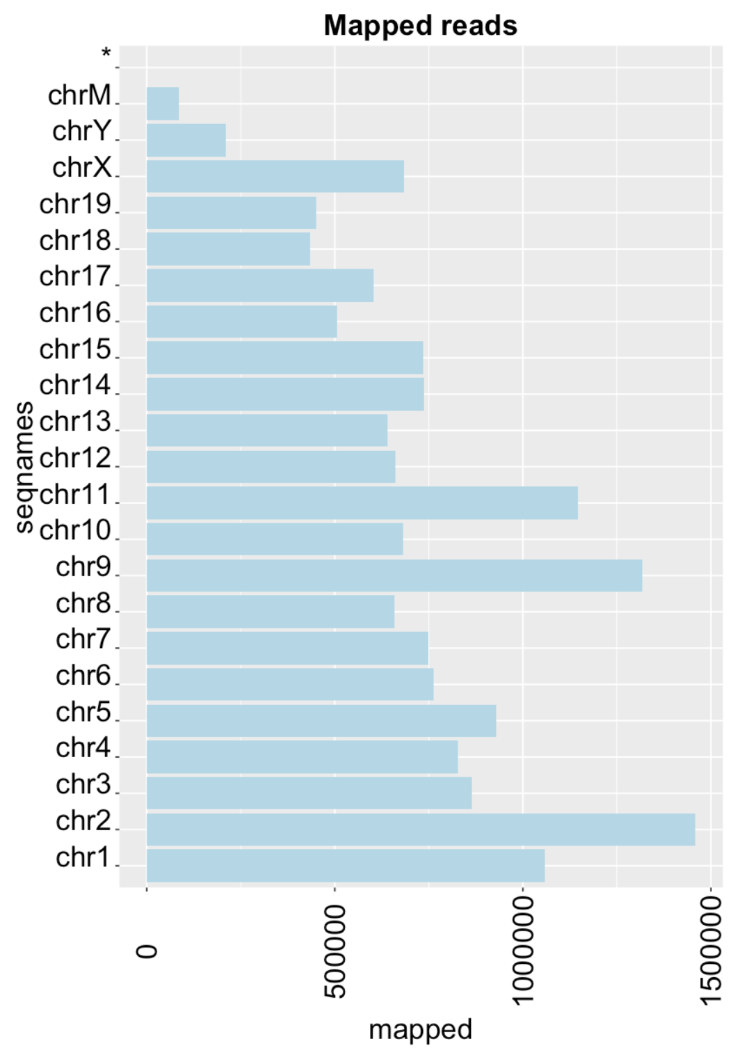
Mapped reads
library(repr)
options(repr.plot.width=9, repr.plot.height=15)
mappedReads <- idxstatsBam("/Users/alexeyefanov/Desktop/Programming/Bioconductor/ChiP-seq/MEL/data/sam/filt_rep1_sorted.bam")
TotalMapped <- sum(mappedReads[, "mapped"])
ggplot(mappedReads, aes(x = seqnames, y = mapped)) + geom_bar(stat = "identity") +
    coord_flip()+
theme(axis.text.x = element_text(color = "black", size = 20, angle = 90, hjust = .5, vjust = .5, face = "plain"),
        axis.text.y = element_text(color = "black", size = 20, angle = 0, hjust = 1, vjust = 0, face = "plain"),
        axis.title.x = element_text(color = "black", size = 15, angle = 0, hjust = .5, vjust = 0, face = "plain"),
        axis.title.y = element_text(color = "black", size = 15, angle = 90, hjust = .5, vjust = .5, face = "plain"))
Creating BigWig and visualizing mapped reads usin IGV
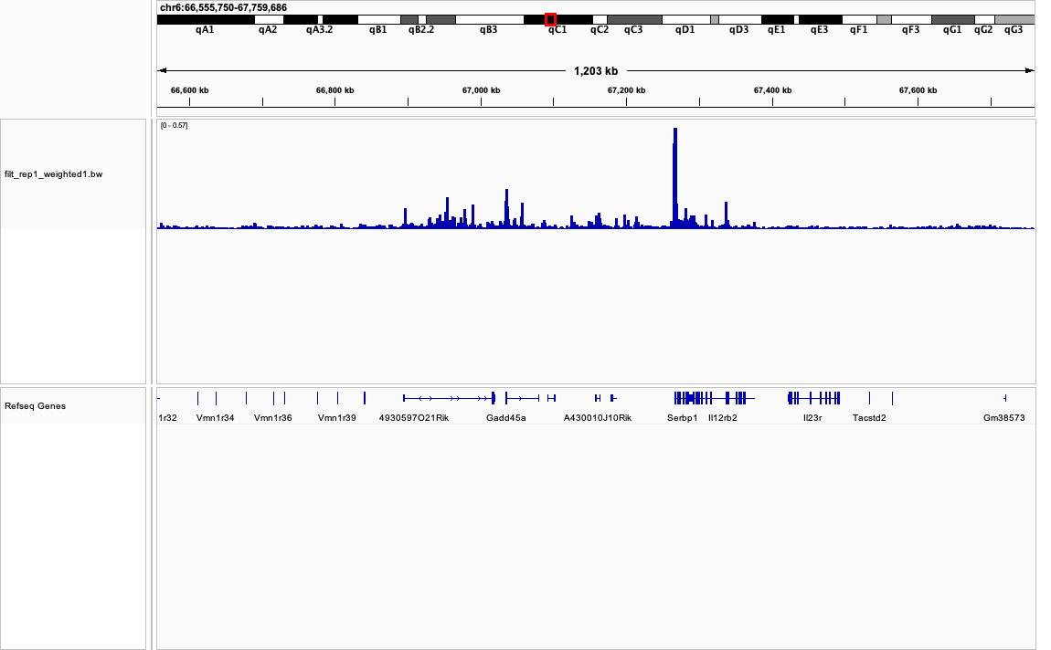
The bigWig format is used to display genomics data in such tools as the UCSC Genome Browser, and The Integrative Genomics Viewer (IGV) as a graph.
BigWig <- coverage("/Users/alexeyefanov/Desktop/Programming/Bioconductor/ChiP-seq/MEL/data/sam/filt_rep1_sorted.bam", weight = (10^6)/TotalMapped)
library(rtracklayer)
export.bw(BigWig, con = "/Users/alexeyefanov/Desktop/Programming/Bioconductor/ChiP-seq/MEL/data/sam/filt_rep1_weighted1.bw")
Downloading output of macs2
macsPeaks <- "/Users/alexeyefanov/Desktop/Programming/Bioconductor/ChiP-seq/MEL/data/peaks/mel_peaks.xls"
macsPeaks_DF <- read.delim(macsPeaks, comment.char = "#")
macsPeaks_DF[1:2, ]
                                            A data.frame: 2 × 10
   chr    start     end length  abs_summit  pileup  X.log10.pvalue. fold_enrichment X.log10.qvalue.  name

1 chr1  4785344 4785933    590     4785600   29.56         14.49350         5.46755        11.17909  mel_peak_1
2 chr1  5083013 5083207    195     5083083   35.06         11.00655         3.60638         7.87681  mel_peak_2
Converting MACS peaks to GRanges object
library(GenomicRanges)
macsPeaks_GR <- GRanges(seqnames = macsPeaks_DF[, "chr"], IRanges(macsPeaks_DF[,
    "start"], macsPeaks_DF[, "end"]))
macsPeaks_GR
GRanges object with 26241 ranges and 0 metadata columns:
          seqnames            ranges strand

      [1]     chr1   4785344-4785933      *
      [2]     chr1   5083013-5083207      *
      [3]     chr1   5677542-5677817      *
      [4]     chr1   6012559-6012715      *
      [5]     chr1   7397544-7398143      *
      ...      ...               ...    ...
  [26237]     chrY 58550402-58550723      *
  [26238]     chrY 60505268-60505555      *
  [26239]     chrY 89932367-89932501      *
  [26240]     chrY 90818621-90818899      *
  [26241]     chrY 90824605-90824835      *
  -------
  seqinfo: 21 sequences from an unspecified genome; no seqlengths
table(seqnames(macsPeaks_GR))
 chr1 chr10 chr11 chr12 chr13 chr14 chr15 chr16 chr17 chr18 chr19  chr2  chr3
 1506  1332  2635  1018  1007   790  1167   852  1304   700   961  1924  1357
 chr4  chr5  chr6  chr7  chr8  chr9  chrX  chrY
 1567  1840  1261  1602  1197  1489   716    12
Adding metadata
mcols(macsPeaks_GR) <- macsPeaks_DF[, c("abs_summit", "fold_enrichment")]
macsPeaks_GR
Filtering out regions overlaping with blacklisted regions
Blacklisted regions are regions showing anomalous read mapping to them.
toBlkList <- "/Users/alexeyefanov/Desktop/Programming/Bioconductor/ChiP-seq/blacklist/ENCFF547METmm10.bed"
blkList <- import.bed(toBlkList)
macsPeaks_GR <- macsPeaks_GR[!macsPeaks_GR %over% blkList]
macsPeaks_GR
GRanges object with 26237 ranges and 2 metadata columns:
          seqnames            ranges strand | abs_summit fold_enrichment
                         |
      [1]     chr1   4785344-4785933      * |    4785600         5.46755
      [2]     chr1   5083013-5083207      * |    5083083         3.60638
      [3]     chr1   5677542-5677817      * |    5677571         5.65644
      [4]     chr1   6012559-6012715      * |    6012601         5.69169
      [5]     chr1   7397544-7398143      * |    7397789         8.75376
      ...      ...               ...    ... .        ...             ...
  [26233]     chrY 58550402-58550723      * |   58550543        17.33837
  [26234]     chrY 60505268-60505555      * |   60505432         8.35447
  [26235]     chrY 89932367-89932501      * |   89932468         5.10398
  [26236]     chrY 90818621-90818899      * |   90818649         3.21887
  [26237]     chrY 90824605-90824835      * |   90824624         2.55565
  -------
  seqinfo: 21 sequences from an unspecified genome; no seqlengths
Peak annotation
The peakAnno object contains the information on annotation of individual peaks to genes.
peakAnno <- annotatePeak(macsPeaks_GR, tssRegion = c(-500, 500), TxDb = TxDb.Mmusculus.UCSC.mm10.knownGene,
    annoDb = "org.Mm.eg.db")
peakAnno
Annotated peaks generated by ChIPseeker
26237/26237  peaks were annotated
Genomic Annotation Summary:
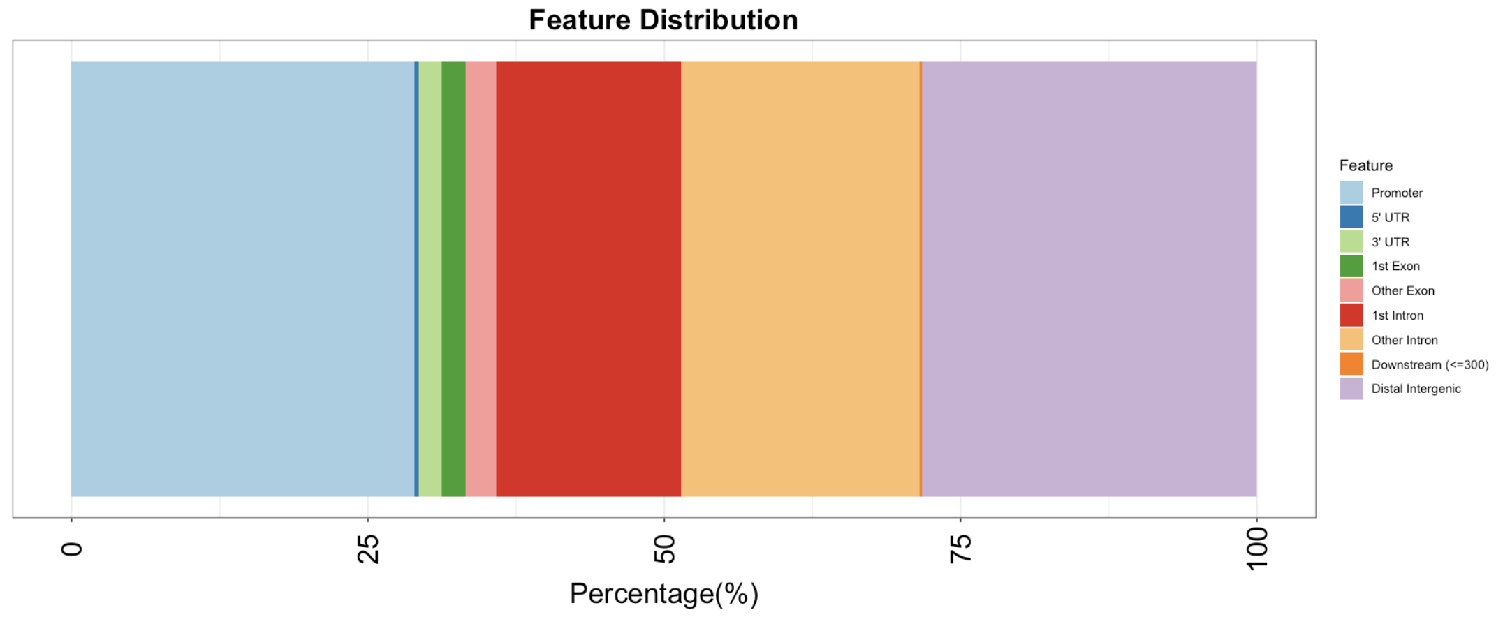
             Feature  Frequency
9           Promoter 28.9514807
4             5' UTR  0.3163471
3             3' UTR  1.9781225
1           1st Exon  2.0048024
7         Other Exon  2.5803255
2         1st Intron 15.5772383
8       Other Intron 20.1433091
6 Downstream (<=300)  0.2210619
5  Distal Intergenic 28.2273126
Converting the peakAnno object to GRanges and Data frame objects
peakAnno_GR <- as.GRanges(peakAnno)
peakAnno_DF <- as.data.frame(peakAnno)
Visualizing of peak annotation
options(repr.plot.width=15, repr.plot.height=6)
plotAnnoBar(peakAnno)+
theme(axis.text.x = element_text(color = "black", size = 20, angle = 90, hjust = .5, vjust = .5, face = "plain"),
        axis.text.y = element_text(color = "black", size = 20, angle = 0, hjust = 1, vjust = 0, face = "plain"),
        axis.title.x = element_text(color = "black", size = 20, angle = 0, hjust = .5, vjust = 0, face = "plain"),
        axis.title.y = element_text(color = "black", size = 20, angle = 90, hjust = .5, vjust = .5, face = "plain"),
     plot.title = element_text(size=20, hjust = .5, vjust = .5, face="bold"))
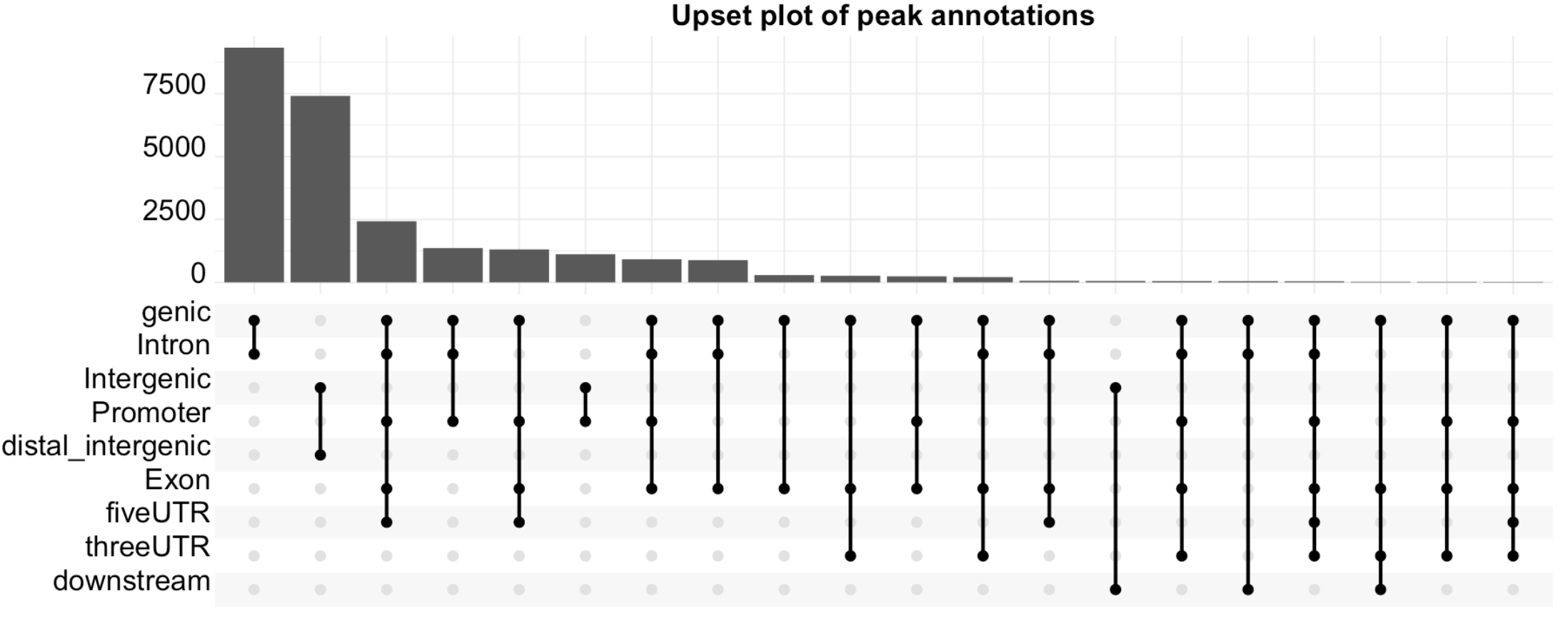
plotDistToTSS(peakAnno)+theme(axis.text.x = element_text(color = "black", size = 20, angle = 90, hjust = .5, vjust = .5, face = "plain"),
        axis.text.y = element_text(color = "black", size = 20, angle = 0, hjust = 1, vjust = 0, face = "plain"),
        axis.title.x = element_text(color = "black", size = 20, angle = 0, hjust = .5, vjust = 0, face = "plain"),
        axis.title.y = element_text(color = "black", size = 20, angle = 90, hjust = .5, vjust = .5, face = "plain"),
     plot.title = element_text(size=20, hjust = .5, vjust = .5, face="bold"))
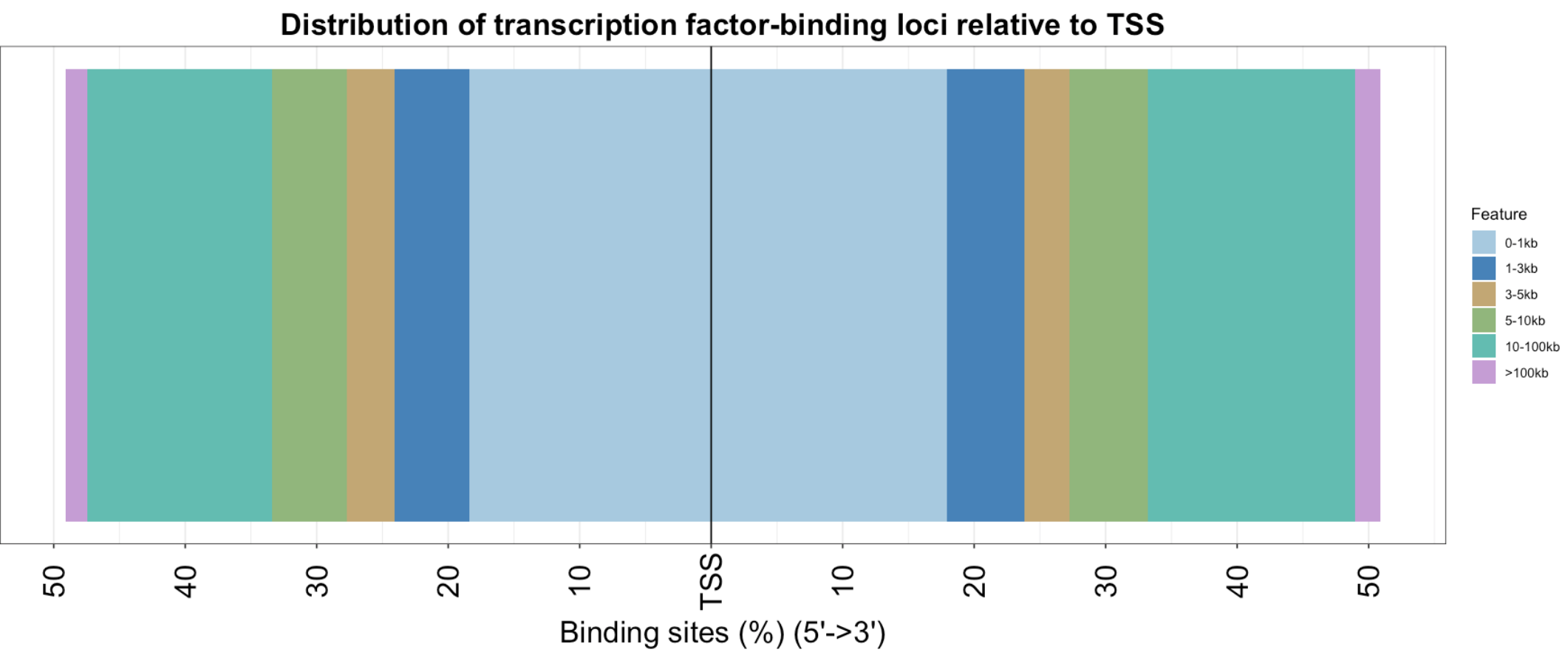
upsetplot(peakAnno, vennpie = F)+theme(axis.text.x = element_text(color = "black", size = 20, angle = 90, hjust = .5, vjust = .5, face = "plain"),
        axis.text.y = element_text(color = "black", size = 20, angle = 0, hjust = 1, vjust = 0, face = "plain"),
        axis.title.x = element_text(color = "black", size = 20, angle = 0, hjust = .5, vjust = 0, face = "plain"),
        axis.title.y = element_text(color = "black", size = 20, angle = 90, hjust = .5, vjust = .5, face = "plain"),
     plot.title = element_text(size=20, hjust = .5, vjust = .5, face="bold"))+ggtitle("Upset plot of peak annotations")
Annotation of peaks to genes
Since transcription factors, as suggested in name, may regulate the transcription of their target genes, we used the ChIPseeker package to associate our peaks, representing potential transcription factor binding events, to their overlapping or closest mm10 genes.
library(TxDb.Mmusculus.UCSC.mm10.knownGene)
library(ChIPseeker)
peakAnno <- annotatePeak(macsPeaks_GR, tssRegion=c(-1000, 1000),
                         TxDb=TxDb.Mmusculus.UCSC.mm10.knownGene,
                         annoDb="org.Mm.eg.db")
Extracting sequences under regions
The motif for the ChIP-ed transcription factor should near the summit (the highest point) of a peak. MEME-ChIP will trim our peaks to a common length internally if sequences are of different length. It is best therefore to provide a peak set resized to a common length.
macsSummits_GR <- GRanges(seqnames(macsPeaks_GR), IRanges(macsPeaks_GR$abs_summit,
    macsPeaks_GR$abs_summit), score = macsPeaks_GR$fold_enrichment)
macsSummits_GR <- resize(macsSummits_GR, 100, fix = "center")
macsSummits_GR
GRanges object with 26237 ranges and 1 metadata column:
          seqnames            ranges strand |     score
                         |
      [1]     chr1   4785550-4785649      * |   5.46755
      [2]     chr1   5083033-5083132      * |   3.60638
      [3]     chr1   5677521-5677620      * |   5.65644
      [4]     chr1   6012551-6012650      * |   5.69169
      [5]     chr1   7397739-7397838      * |   8.75376
      ...      ...               ...    ... .       ...
  [26233]     chrY 58550493-58550592      * |  17.33837
  [26234]     chrY 60505382-60505481      * |   8.35447
  [26235]     chrY 89932418-89932517      * |   5.10398
  [26236]     chrY 90818599-90818698      * |   3.21887
  [26237]     chrY 90824574-90824673      * |   2.55565
  -------
  seqinfo: 21 sequences from an unspecified genome; no seqlengths
Extracting sequences under regions
peaksSequences <- getSeq(BSgenome.Mmusculus.UCSC.mm10, macsSummits_GR)
names(peaksSequences) <- paste0(seqnames(macsSummits_GR), ":", start(macsSummits_GR),
    "-", end(macsSummits_GR))

peaksSequences[1:2, ]
DNAStringSet object of length 2:
    width seq                                               names
[1]   100 CCGCACCGCCGCCAAGCGTTTAC...GGACCGCAGCAGGTCCAGGCTGG chr1:4785550-4785649
[2]   100 TTTGGTGCGCGGTCCAGCAGTTT...CAGACGCTGCTGTCACTTCGTAG chr1:5083033-5083132
Saving the peaksSequences object as meme.fa
The meme.fa file will be feeded into MEME-Chip (the comprehensive motif analysis (including motif discovery) tool)
writeXStringSet(peaksSequences, file ="/Users/alexeyefanov/Desktop/Programming/Bioconductor/ChiP-seq/MEL/data/meme.fa").
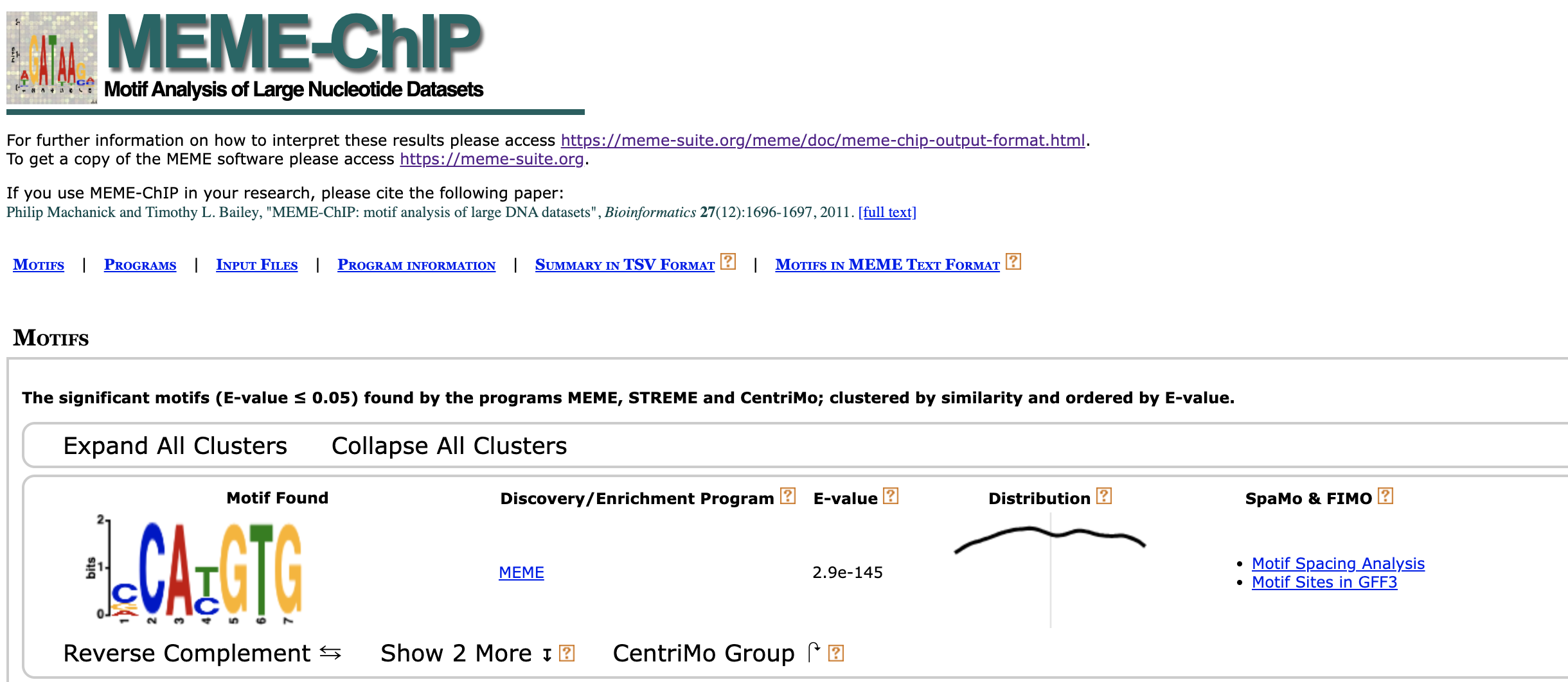
meme-chip -maxw 10 -minw 5 -o results meme.fa
Back to bioinformatics project page: Back to bioinformatics project page
Back to home: Back to home