Projects
Projects' code is stored on GitHub (links are provided).
Current weather
Program Description
The program displays the current weather for a region upon providing a zip code and two letters of a country code without a white space between them. This program has two functions: main() and key(). The main() function has no arguments, and prompts for an address and passes it to the key(address) function. The key(address) function parses site https://openweathermap.org/ for inputted address and returns the current weather data.Program Usage
The program prompts a user to enter a zip code, comma, and two lowercase letters of the country code without a whitespace. After hitting the ENTER button it displays the current weather for the inputted regionExample of output for 101000,ru (Moscow, September 25):
| Weather characteristics | Weather data |
|---|---|
| Cloudiness | scattered clouds |
| Temperature, C | 20 |
| Pressure, hpa | 1020 |
| Humidity, % | 47 |
| Temperature minimal, C | 19 |
| Temperature maximal, C | 20 |
| Visibility, m | 10000 |
| Wind speed, m/s | 4.77 |
| Wind degree | 184 |
| Geocoords | [37.6156, 55.7522] |
Link to GitHub: Link to Github
Back to top: Back to TopWine Type Prediction
The aim of this project is to predict type of the wine-white or red-based on its chemical properties and physical properties. For this project two wine datasets were used that contain information about some chemical components for both the white wine and the red wine. The two analyzed datasets are related to red and white variants of the Portuguese "Vinho Verde" wine. Vinho Verde (pronounced “veeng-yo vaird”) is a Portuguese wine that comes from the region of Vinho Verde. The 10 wine features were included in datasets together with a column containing quality score of each wine (score ranges between 0 and 10). Each dataset contains following features:
- fixed acidity
- volatile acidity
- citric acid
- residual sugar
- chlorides
- free sulfur dioxide
- total sulfur dioxide
- density
- pH
- sulphates
- alcohol
- quality
Logistic regression model was used to predict type of wine (red or white wine) based on wine chemical and physical properties.
Model performance are summarized in the table below:
| precision | recall | f1-score | support | |
|---|---|---|---|---|
| white wine | 0.99 | 0.99 | 0.99 | 1225 |
| red wine | 0.98 | 0.98 | 0.98 | 400 |
accuracy:0.99
Conclusion: The logistic regression model shows a good performance with accuracy=0.99, recall (white wine)=0.99, and recall (red wine)=0.98
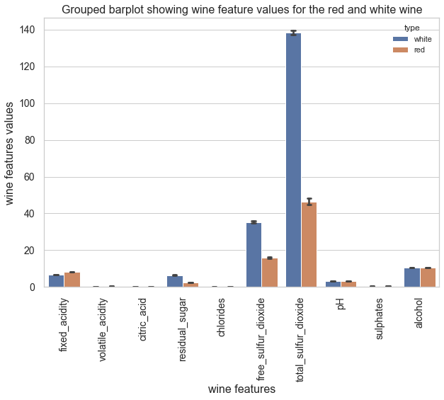
Thw table below shows the ratio between the mean values of red and the mean values white wines. The figure below shows a grouped barplot of the values for each feature of white and red wine
| wine features | ratio of mean values of red and white wines |
|---|---|
| fixed_acidity | 1.213697 |
| volatile_acidity | 1.896990 |
| citric_acid | 0.810839 |
| residual_sugar | 0.397221 |
| chlorides | 1.910903 |
| free_sulfur_dioxide | 0.449612 |
| total_sulfur_dioxide | 0.335845 |
| pH | 1.038531 |
| sulphates | 1.343581 |
| alcohol | 0.991318 |
| quality | 0.958848 |

Conclusion: The most important features to descriminate between white wine and red wine are:
- total sulfur dioxide: about 3 times higher in white wine in comparison with red wine
- residual sugar: about 3 times higher in white wine in comparison with red wine
- chlorides: about 2 times higher in red wine in comparison with white wine
- volatile acidity: about 2 times higher in red wine in comparison with white wine
Back to top: Back to Top
Application of K-Means and DBSCAN to cluster cancer cell lines based on gene expression signature
The goal of this project is to classify (cluster) tumor cell based on gene expression profiling.
Dataset
In the current project, a data set from the US Irvine Machine Learning Repository will be analyzed. That data set contains 881 samples. Each sample derived from one out of five cancer type-PRAD, LUAD, BRCA, KIRS, and COAD. Each sample contains data for expression of 20,551 genes. Thus, the dataframe contains 881 samples and 20,551 columns (features).Methods
- Principle component analysis (PCA) will be used to reduce dimensionality of the data set. Using PCA is important because analyzed dataset has more than 20 thousand features. But the major disadvantage of PCA is that the PCA components are hardly interpretable.
- K-means. The elbow method was used to determine the optimal numbers of k. The silhouette coefficient and the adjusted rand index (ARI) were used to measure the similarity between true and predicted classes using known true classes.
- Density-based Spatial Clustering of Application with Noise (DBSCAN). The elbow method will be used to determine the optimal eps and min_samples values. The silhouette coefficient and the adjusted rand index (ARI) were used to measure the similarity between true and predicted classes using known true classes.
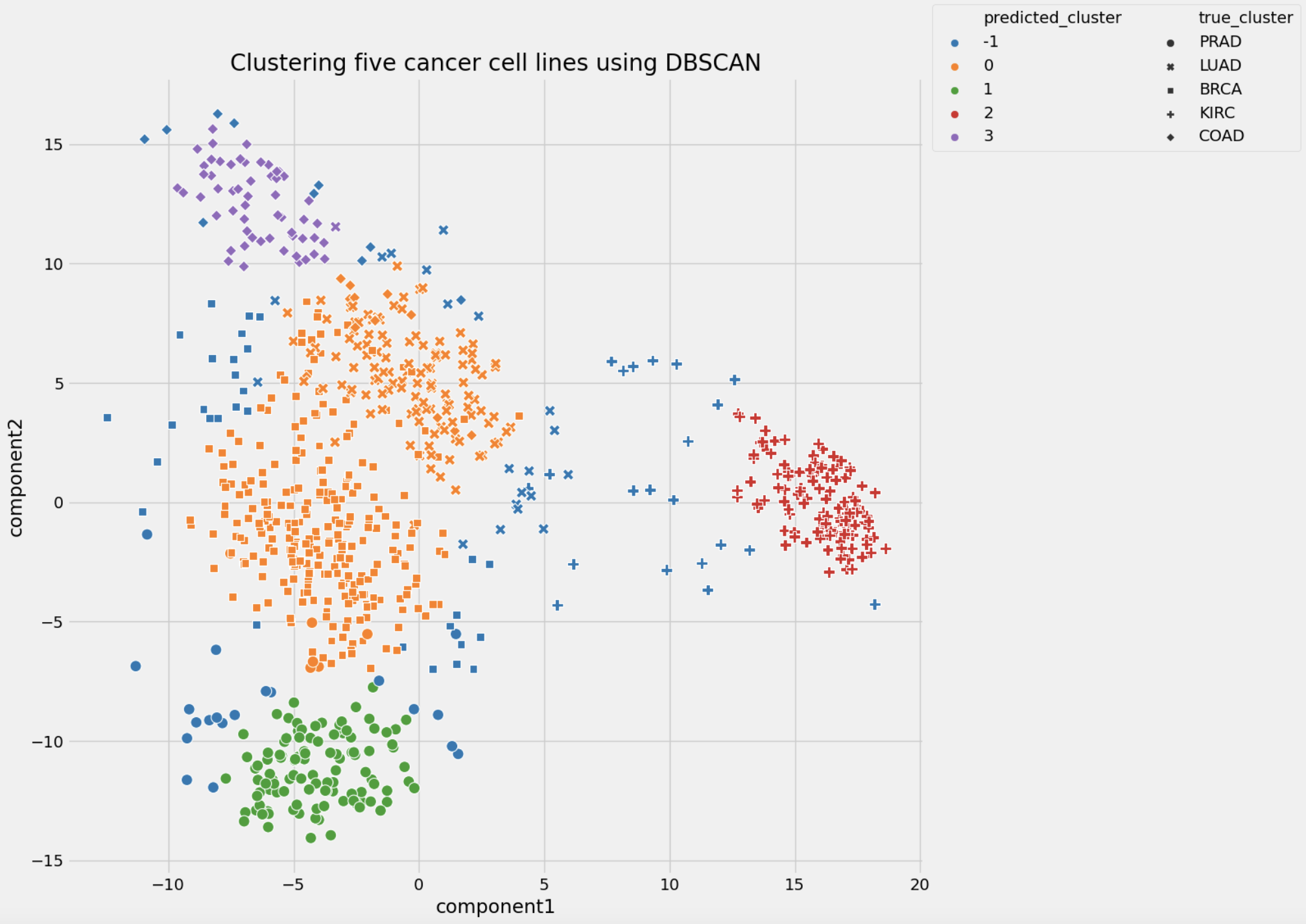
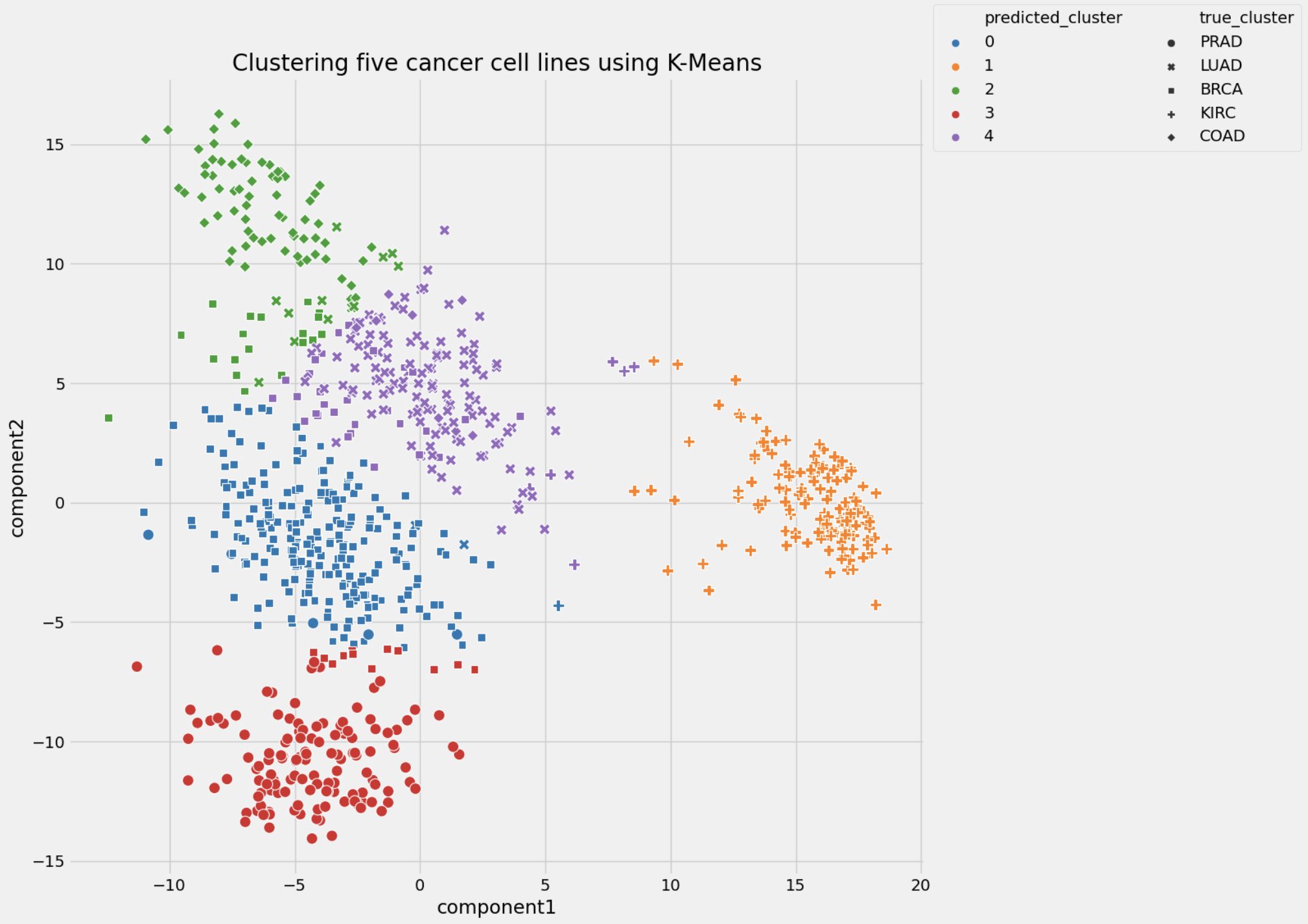
Figures below show clustering performance for DBSCAN and K means


| Performance metrics | k-means | DBSCAN |
|---|---|---|
| silhouette score | 0.512 | 0.722 |
| adjusted rand index | 0.379 | 0.523 |
Conclusion: K-means and DBSCAN algorithms were used to separate analyzed cancer cell lines into clusters based on gene expression signature. The k-means algorithm showed a better performance in comparison with the DBSCAN algorithm:
Thus, cancer cell lines can be clustered based on the gene signature expression.
Link to GitHub: Link to GithubBack to top: Back to Top
Breast Cancer Prediction using different ML algorithms
The following nuclei features have been used for predictions
1. Radius
2. Texture
3. Perimeter
4. Area
5. Smoothness (local variation in radius)
6. Compactness
7. Concavity
8. Concave points
9. Symmetry
10. Fractal Dimension
The following ML algorithms were used in the current project: Logistic Regression, KNN,Naive Bayes, Decision Tree, Random Forest, SVM. Results are summarized in the table:
| Model performance | Logistic Regression | KNN | Naive Bayes | Decision Tree | Random Forest | SVM |
|---|---|---|---|---|---|---|
| recall (benign) | 1.00 | 0.99 | 0.89 | 0.89 | 0.91 | 0.98 |
| recall (malignant) | 0.89 | 0.91 | 0.89 | 0.96 | 0.94 | 0.89 |
| accuracy | 0.96 | 0.96 | 0.89 | 0.92 | 0.92 | 0.94 |
Conclusion:The highest accuracy (0.96) show the logistic regression model and knn, while highest recall (malignant tumor) 0.96 shows the decision tree model. Since the goal is to predict breast cancer that the decision tree model shows the best performance in terms of prediction malignant tumor
Link to GitHub: Link to GithubBack to top: Back to Top
Prediction of Heart Disease

This data set contains 4000 records and 16 variables. These 16 variables describe each participant of this study. The purpose of this case study is to investigate whether there is a risk of coronary heart disease within 10 years given such variables. This data set contains following variables:
Demographic:
- Sex of a participant male or female. 0-female. 1-male
- Age. This variable is expressed in whole numbers
- Education
-
Behavioral:
- currentSmoker. 0-non-smoker, 1-smoker
- cigsPerDay. This variable describes the number of cigarettes per day. Interval 0-20
-
Medical history:
- BPmeds: whether or not the patient was on blood pressure medication, 0-no, 1-yes
- prevalentStroke: whether or not the patient had previously had a stroke, 0-no, 1-yes
- prevalentHyp: whether or not the patient was hypertensive, 0-no, 1-yes
- diabetes: whether or not the patient had diabetes, 0-no, 1-yes
- Medical(current):
- totChol:total cholesterol level
- sysBP: systolic blood pressure
- diaBP: diastolic blood pressure
- BMI: Body Mass Index
- heartrate: heart rate
- glucose: glucose level
The logistic regression model was used in the current project to predict whether the heart disease occur within 10 years based on features listed above. Initially, model had a poor performance in terms of heart disease prediction, but after hyperparameter tuning the performance was greatly improved as shown in table below
| Model performance | Default threshold 0.5 | The best threshold 0.14 | recall (no heart disease) | 0.99 | 0.64 | recall (heart disease) | 0.09 | 0.73 |
|---|
Conclusion:Using the best threshold obtained from ROC curve greatly improved the model performance in terms of heart disease prediction with recall=0.73
Link to GitHub: Link to Github
Back to top: Back to Top
Credit card fraud detection
The goal of this project is to build a few ML models, select the best one and select several the most important features in predicting fraud.
Decision Tree, Random Forest, and Logistic regression were used to build models.
In the current project, a data set from the US Irvine Machine Learning Repository will be analyzed. The data set includes transactions made by credit cards during two days in September 2013 in Europe. There are totally 284,807 transactions. Among these transactions 492 are fraudulent. The dataset is highly imbalanced because fraudulent transactions account for 0.172% of all transactions.
The data set contains totally 31 variables. 28 variables are the result of a PCA transformation. Unfortunately, due to confidentiality issues, the original features are not provided. Two feature variables 'Time' and 'Amount' are not transformed by PCA. Feature 'Time' contains the seconds elapsed between each transaction and the first transaction in the dataset. The ‘Time’ variable is irrelevant to the current study and was deleted from the data frame. The feature 'Amount' is the transaction amount. The variable 'Class' is the target variable and it takes value 1 in case of fraud and 0 otherwise. Model performance characteristics are shown in the table below:
| Model performance | Logistic Regression | Decision Tree | Random Forest |
|---|---|---|---|
| recall (no fraud) | 0.96 | 1 | 1 |
| recall (fraud) | 0.91 | 0.83 | 0.78 |
| accuracy | 0.96 | 1 | 1 |
Conclusion The best performance to detect credit card fraud showed the logistic regression model with threshold 0.001644 The six top important features to detect fraud are V4, V10, V14, V20, V9, V17
Link to GitHub: Link to GithubBack to top: Back to Top
Collecting historical weather data from different sources for 9 years and evaluating trends

For this project I choose 3 historical data sets for the US zip 43212 (Columbus, Ohio). The first data set I downloaded from https://www.worldweatheronline.com/ (in csv format). The data contains historical weather data from 07/01/2008 to 10/25/2020 in hourly basis. I selected only data for noon for each day. Next, historical weather data from 09/30/2011 to 09/29/2014 were extracted.
The dataset was split on three parts- 09/30/2011-09/29/2012
- 09/30/2012-09/29/2013
- 09/30/2013-09/29/2014
The second dataset was downloaded from https://openweathermap.org again in csv format. I created the html format from the csv file. The html file contains historical weather data from 09/29/2014 to 09/29/2017.
The dataset was split on three parts- 09/30/2014-09/29/2015
- 09/30/2015-09/29/2016
- 09/30/2016-09/29/2017
The third data set was downloaded from https://www.visualcrossing.com
- 09/30/2019-09/29/2020
- 09/30/2018-09/29/2019
- 09/30/2017-09/29/2018
The whole idea of this project is to compare temperature for 9 consecutive periods and evaluate temperature trends
Link to GitHub: Link to Github