scRNA-seq

Project description

The current project is aimining to reanalyze data published at the paper: Epigenetic regulation of white adipose tissue plasticity and energy metabolism by nucleosome binding HMGN proteins.
Link to the paper: link
In that paper, authors investigated the role HMGNs in white adipocyte browning. They employed scRNAseq to achieve that goal. WT mice (control) were compared with DKO mice. DKO mice are genetically modified mice that are lacking HMGN1 and HMGN2 proteins. Two bilogical replicates of each line were used at two time points-0 days and 6 days. Totally 8 samples were used in that study. Table below shows sample names and experiment conditions:

Sample	Species	Condition	Time Point	Replicate	Status
W10	Mouse	WT	0	1	Preadipocyte
W20	Mouse	WT	0	2	Preadipocyte
D10	Mouse	DKO	0	1	Preadipocyte
D20	Mouse	DKO	0	2	Preadipocyte
W16	Mouse	WT	6	1	Adipocytes
W26	Mouse	WT	6	2	Adipocytes
D16	Mouse	DKO	6	1	Adipocytes
D26	Mouse	DKO	6	2	Adipocyte

Raw data downloding and reads mapping

scRNAseq sra files (PRJNA796303) can be accessed at link to raw data
The tsv table was downloaded from ENA: PRJNA796303_tsv.txt. Links to sra files were extracted from that file by code:

awk 'NR>1{print $9}' PRJNA796303_tsv.txt | awk '{gsub(/\;/,"\n")};{print $0}' >download3.sh

The download3.sh file contained following links:

ftp.sra.ebi.ac.uk/vol1/srr/SRR175/087/SRR17555087
ftp.sra.ebi.ac.uk/vol1/srr/SRR175/088/SRR17555088
ftp.sra.ebi.ac.uk/vol1/srr/SRR175/090/SRR17555090
ftp.sra.ebi.ac.uk/vol1/srr/SRR175/083/SRR17555083
ftp.sra.ebi.ac.uk/vol1/srr/SRR175/084/SRR17555084
ftp.sra.ebi.ac.uk/vol1/srr/SRR175/086/SRR17555086
ftp.sra.ebi.ac.uk/vol1/srr/SRR175/089/SRR17555089
ftp.sra.ebi.ac.uk/vol1/srr/SRR175/085/SRR17555085 

sra files were downloaded by following command:

wget -i download3.sh 

Next, each sra file was split on 3 files:

for sample in $(cat /data/mice/PRJNA796303/unique_samples); do 
fastq-dump --split-files --gzip $sample --outdir /data/mice/PRJNA796303/rawData
 done 

3 files correspond to each sample:
R1-barcode +UMI
R2-insert
I-sample index

cellranger was used to map reads to mouse genome:

for sample in $(cat /data/mice/PRJNA796303/unique_samples); do 
cellranger count --id=$sample \
   --fastqs=/data/mice/PRJNA796303/rawData \
   --sample=$sample \
   --no-bam \
   --transcriptome=/data/mice/PRJNA796303/refdata-gex-GRCm39-2024-A;
done 

unique_samples contains following names:
SRR17555083
SRR17555084
SRR17555085
SRR17555086
SRR17555087
SRR17555088
SRR17555089
SRR17555090

cell ranger output files were transferred to local computer and analyzed in Seurat 5.1.0 (Bioconductor 3.19)

Analysis aligned data in Seurat

Loading required libraries

library(SCINA)
library(cerebroApp)
library(msigdb)
library(scmap)
library(celldex)
library(SingleR)
library(Seurat)
library(hdf5r)
library(gdata)
library(Matrix)
library(DropletUtils)
library(patchwork)
library(harmony)
library(SoupX)
library(glmnet)
library(ComplexHeatmap)
library(ggplot2)
library(dplyr)
library(EBImage)
library(glmGamPoi)
library(tibble)
library(repr)
library(purrr)

Generally, cellranger output files can be read into Seurat with two methods Read10X() and Read10X_h5(). The Read10X() accepts data from the filtered_feature_bc_matrix folder. That folder has 3 files: barcodes.tsv.gz, features.tsv.gz, and matrix.mtx.gz. The Read10X_h5() method accepts data in Hierarchical Data Format 5 (HDF5). This data format is designed to store large amount of data. I use the Read10X_h5() method. The hdf5r package reads hdf5 files. First, we need to get list of all .h5 files in the output directory:

files <- list.files(path="/Users/alexeyefanov/Desktop/Programming/biobase/GSE193462/output",recursive=T,pattern="*.h5")
files

'D10/filtered_feature_bc_matrix.h5''D16/filtered_feature_bc_matrix.h5'
'D20/filtered_feature_bc_matrix.h5''D26/filtered_feature_bc_matrix.h5'
'WT10/filtered_feature_bc_matrix.h5''WT16/filtered_feature_bc_matrix.h5'
'WT20/filtered_feature_bc_matrix.h5''WT26/filtered_feature_bc_matrix.h5'

Reading hdf5 files (extension .h5)

The h5_read is the list of matrices.

h5_read <- lapply(paste0("/Users/alexeyefanov/Desktop/Programming/biobase/GSE193462/output/", files), Read10X_h5)

Next step is creating the Seurat object. The Seurat object is used to store the raw count matrices (located in h5_read), metadata, and processed data, plots etc. The CreateSeuratObject() method is used to create the Seurat object. This object has several arguments including min.cells and min.features. For example, min.cells = 3 will filter out genes that are present in less than 3 cells. min.features=200 will filter out cells containing less than 200 expressed genes. To create the Seurat object we assign names to matrices

names(h5_read)<- sapply(files, 
                        function(x){str_split_1(x,"/")[1]}
                        )
names(h5_read)

'D10''D16''D20''D26''WT10''WT16''WT20''WT26'

Creating Seurat object

adp <- mapply(CreateSeuratObject,counts=h5_read,  
              project=names(h5_read),
              MoreArgs = list(min.cells = 3, min.features = 200))

The adp object is a list of 8 seurat objects. To further proceed with analysis all seurat objects should be merged. There is a potential problem with merging seurat objects since cell barcodes can overlap between different samples and duplicated barcodes will be dropped. To avoid it the add.cell.id argument should be used. The add.cell.id argument value will be added to barcode name. The simplest way is to set up the add.cell.id argument's value equals to sample name.

Merge Seurat objects

adp <- merge(adp[[1]], y = adp[2:length(adp)], 
                  add.cell.ids = names(adp),project="Adipose")
adp
 

An object of class Seurat 
24912 features across 49138 samples within 1 assay 
Active assay: RNA (24912 features, 0 variable features)
8 layers present: counts.D10, counts.D16, counts.D20, counts.D26, counts.WT10, counts.WT16, counts.WT20, counts.WT26

The adp object has 13 slots:

 slotNames(adp)

 'assays''meta.data''active.assay''active.ident''graphs''neighbors''reductions''images''project.name''misc''version''commands''tools'

Each slot can be accessed using @ notation, for example:

 adp@assays

 $RNA
Assay (v5) data with 24912 features for 49138 cells
First 10 features:
Xkr4, Gm1992, Gm19938, Rp1, Sox17, Mrpl15, A930006A01Rik, Lypla1,
Tcea1, Rgs20 
Layers:
counts.D10, counts.D16, counts.D20, counts.D26, counts.WT10,
counts.WT16, counts.WT20, counts.WT26

meta.data is a slot of the seurat object and can be accessed through @ notation.

head(adp@meta.data)

                    A data.frame: 6 × 3
                        orig.ident   nCount_RNA  nFeature_RNA
  
D10_AAACCCAAGATGCTTC-1         D10        13602          4182
D10_AAACCCAAGCTCTTCC-1         D10        38649          6789
D10_AAACCCAAGTCATCGT-1         D10        31695          5694
D10_AAACCCAGTAGCGTCC-1         D10        21310          4959
D10_AAACCCAGTGCACGCT-1         D10        28390          4977
D10_AAACCCAGTGTAAATG-1         D10         5835          2276

orig.ident - sample's labels
nCount_RNA - number of UMIs per cell
nFeature_RNA - number of genes expressed (detected) per cell

the meta.date data frame should be updated with type of mice (condition) and time points (time_point) information. The combination of condition and time_point will be added as well.

adp$condition <- ifelse(str_detect(adp@meta.data$orig.ident, "^W"),
                        "WT","DKO")
adp$time_point <- ifelse(str_detect(adp@meta.data$orig.ident, "0"),
                         "Day 0","Day 6")
adp$cond_tp <- paste(adp$condition, adp$time_point)

Visualization of the number of cells per sample

 adp@meta.data %>% 
  ggplot(aes(x=orig.ident, fill=orig.ident)) + 
  geom_bar(color="black") +

  stat_count(geom = "text", colour = "black", size = 3.5, 
            aes(label = after_stat(count)),
            position=position_stack(vjust=0.5))+

  theme_classic() +
  theme(plot.title = element_text(hjust=0.5, face="bold")) +
  ggtitle("Number of Cells per Sample")
ggsave("seurat_barplot.png")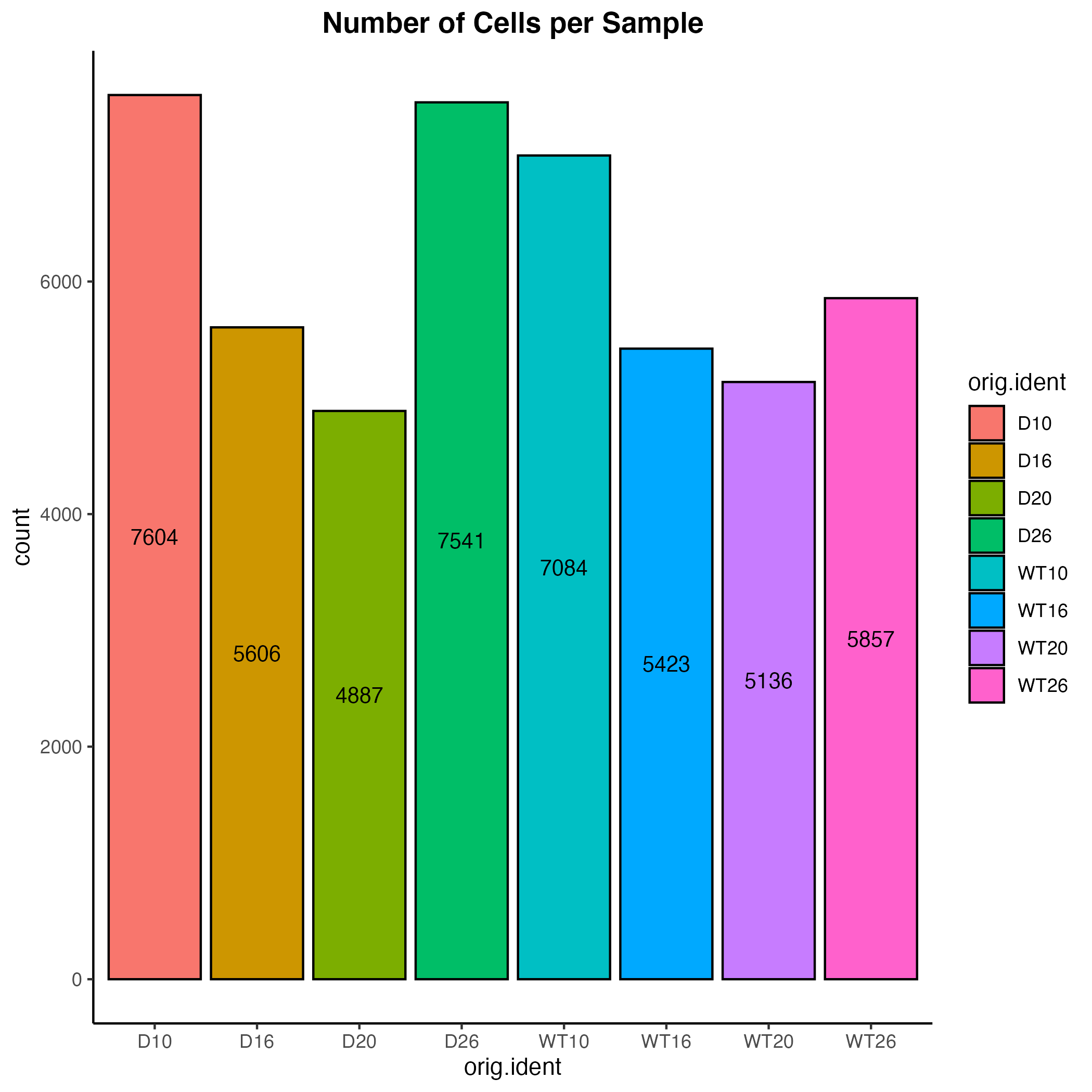

Saving adp object in R Data Serialization (RDS) format

saveRDS(adp,"/Users/alexeyefanov/Desktop/Programming/biobase/GSE193462/output/merged_Seurat_adp1.rds")

Quality Control

There are 3 main QC metrics:

• nCount_RNA
• nFeature_RNA
• percent.mt: the fraction of reads from mitochondrial genes per cell

Addition percent.mt to mata.data

adp[["percent.mt"]] <- PercentageFeatureSet(adp, pattern = "^mt-")
metadata <- adp@meta.data

The percent.mt thresholds will be set up based on visualization of percent.mt in WT and DKO mice

cnames<-setNames(rep(c("cyan3","darkgoldenrod1"),each=4),levels(factor(metadata$orig.ident))) 
levels(factor(metadata$orig.ident))
cnames 

'D10''D16''D20''D26''WT10''WT16''WT20''WT26'
D10'cyan3'D16'cyan3'D20'cyan3'D26'cyan3'WT10'darkgoldenrod1'WT16'darkgoldenrod1'WT20'darkgoldenrod1'WT26'darkgoldenrod1' 

 VlnPlot(adp, features = "percent.mt", group.by="orig.ident") +
  scale_fill_manual(values=cnames) +
  geom_hline(yintercept=10,color="red")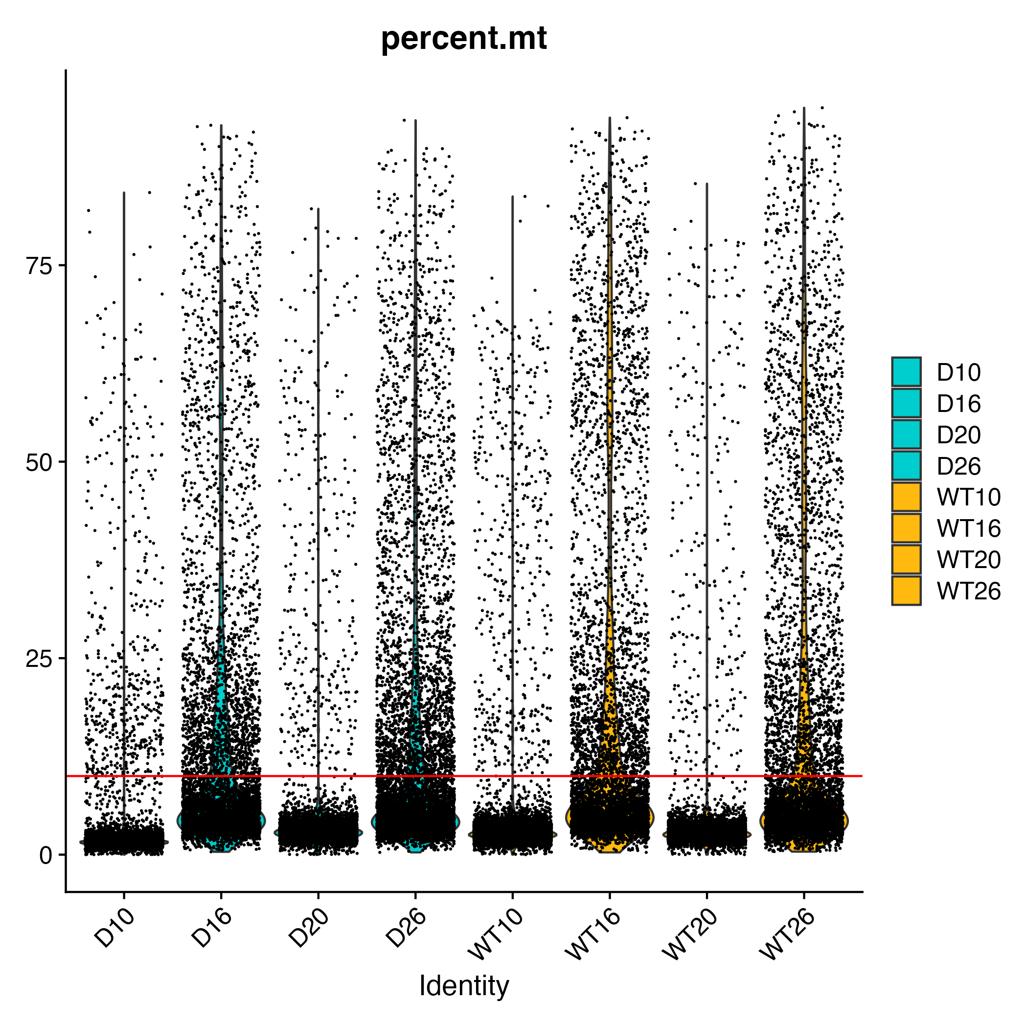

Selected filtration criteria:
Day 0:
nFeature_RNA > 350
nCount_RNA >650
percent.mt <10
Day 6:
nFeature_RNA > 350
nCount_RNA >650
percent.mt <25

t0<- metadata |> filter(time_point=="Day 0", nFeature_RNA > 350, 
                        nCount_RNA >650, percent.mt <10 ) |> 
  rownames_to_column("Cell") |> pull(Cell) 

t6<- metadata |> filter(time_point=="Day 6", nFeature_RNA > 350, 
                        nCount_RNA >650, percent.mt <25 ) |> 
  rownames_to_column("Cell") |> pull(Cell)

keep<-c(t0,t6)

Filtering the seurat object

 adp_filt<-subset(adp, cells=keep)

Saving the adp_filt object in R data serialization (rds) format.

saveRDS(adp_filt,"/Users/alexeyefanov/Desktop/Programming/biobase/GSE193462/output/adp_merge_filt1.rds")

Normalization

library(sctransform)
library(glmGamPoi)
adp_filt<-readRDS("/Users/alexeyefanov/Desktop/Programming/biobase/GSE193462/output/adp_merge_filt_sctran_clust0.1.rds")
 

Linear Dimensionality Reduction

adp_filt <- RunPCA(adp_filt, verbose = FALSE, assay="SCT")
 

Exploring the PCA results

options(repr.plot.width=10, repr.plot.height=10)
ElbowPlot(adp_filt, ndims = 40)
ggsave("elbow.jpg")
 

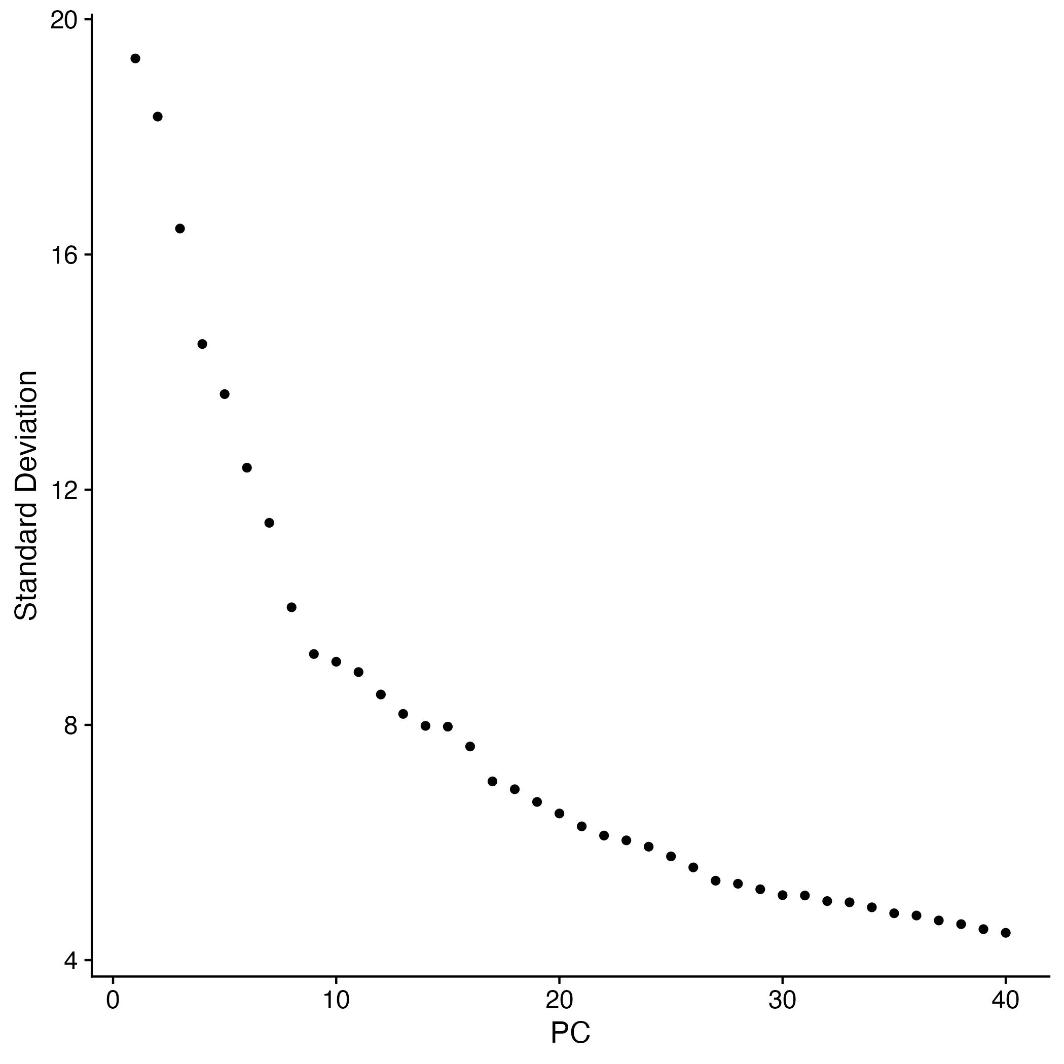
The majority of variation is captured by around 30 PC.

Clustering

adp_filt <- FindNeighbors(adp_filt, dims = 1:30)
adp_filt <- FindClusters(adp_filt, resolution = 0.1)
 

The above commands create the SCT_snn_res.0.1 and seurat_clusters columns in meta.data.

Modularity Optimizer version 1.3.0 by Ludo Waltman and Nees Jan van Eck

Number of nodes: 42502
Number of edges: 1423435

Running Louvain algorithm...
Maximum modularity in 10 random starts: 0.9509
Number of communities: 9
Elapsed time: 8 seconds
 

Cluster visualization using uniform manifold approximation and projection (UMAP)

adp_filt <- RunUMAP(adp_filt,dims = 1:30)
 

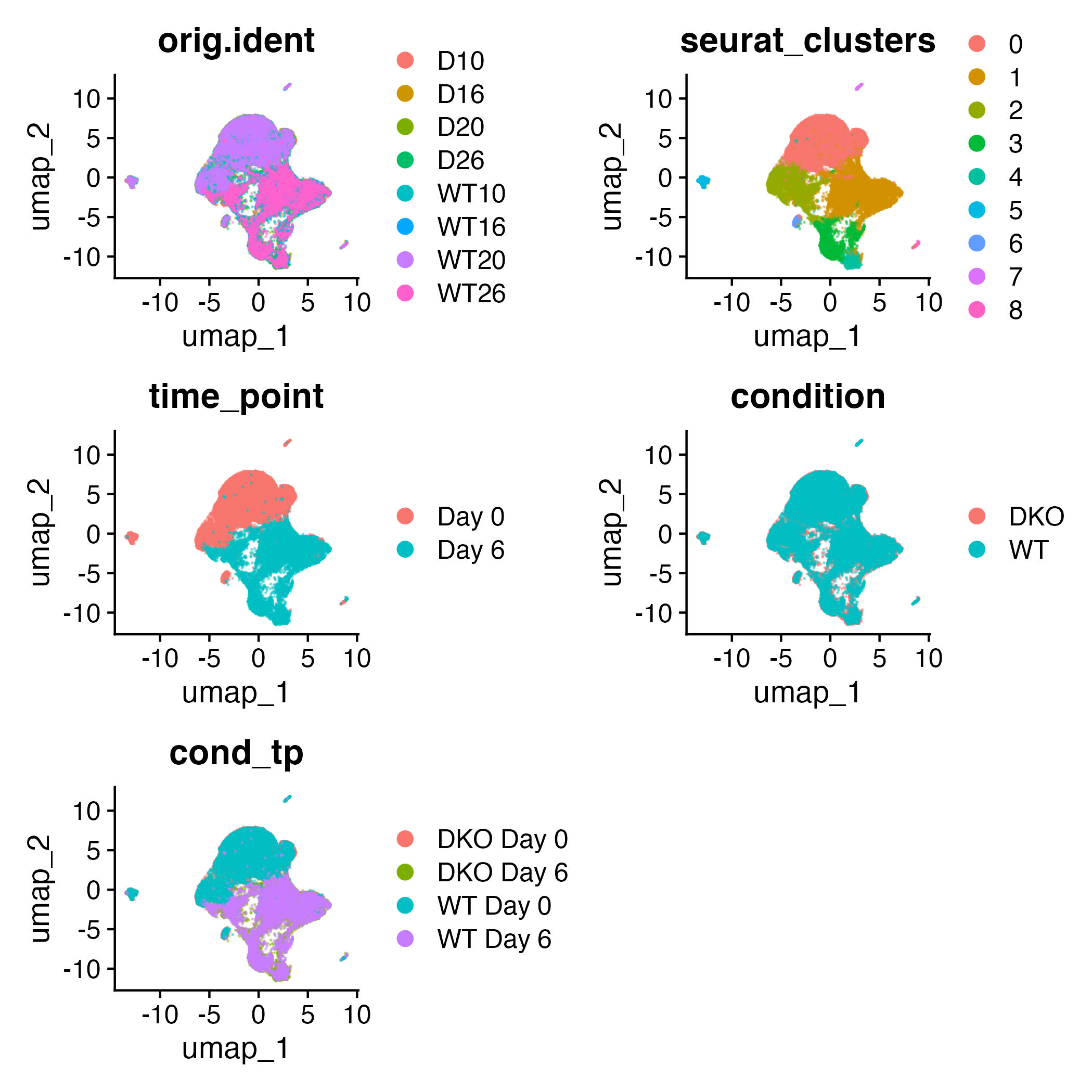
Visualizing potential contamination

Ptprc (CD45+): nucleated hematopoietic cells
Pecam: endothelial cells
Plp1:neuronal and glial cells

contam=c("Ptprc", "Plp1", "Pecam1")
VlnPlot(adp_filt, features=contam)
ggsave("contam.jpg")
FeaturePlot(adp_filt,features=contam)
ggsave("contam_cluster.jpg")
 

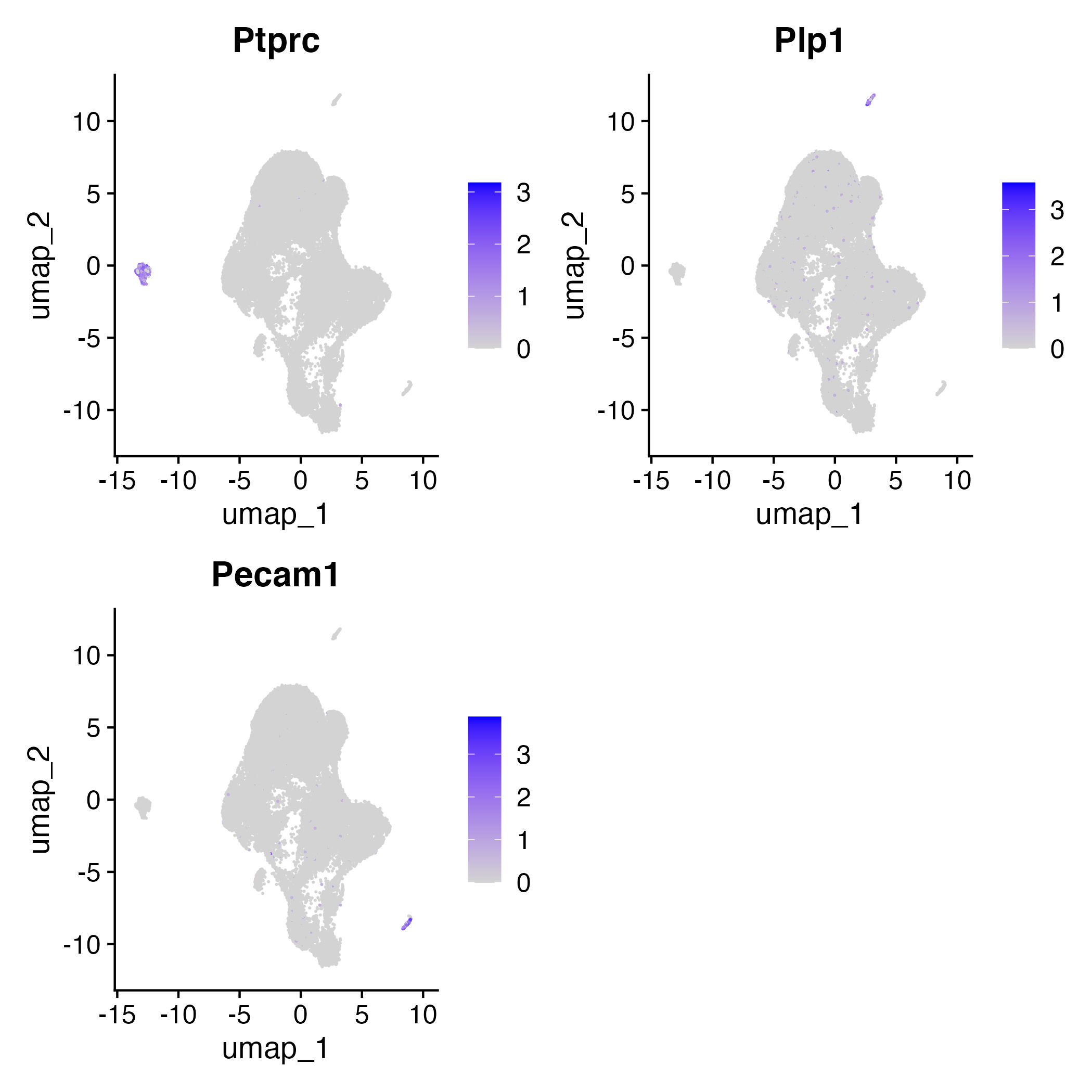
Removal clusters with high contaminations of Ptprc, Plp1, and Pecam1

adp<-adp_filt
Idents(adp) = "SCT_snn_res.0.1"
`%not_in%` <- purrr::negate(`%in%`)
adp <- subset(adp, subset=seurat_clusters %not_in% c(5,7, 8))
 

Finding Cluster Biomarkers

adp<-PrepSCTFindMarkers(adp, verbose=T)
Idents(adp) = "SCT_snn_res.0.1"
DefaultAssay(adp) = "SCT"
de_allClusters = FindAllMarkers(adp, test.use="wilcox", min.pct=0.1, logfc.threshold = 0.25, only.pos=TRUE)
 

Selecting 5 top differentially expressed (DE) genes in all clusters

 de_allClusters %>%
    group_by(cluster) %>%
    dplyr::filter(avg_log2FC > 1) %>%
    slice_head(n = 5) %>%
    ungroup() -> top5
head(top5)
 

Heatmap of 5 top DE genes for each cluster

options(repr.plot.width=8, repr.plot.height=8)
DoHeatmap(adp,features = top5$gene, slot="scale.data")
ggsave("doheatmap.jpg")
 

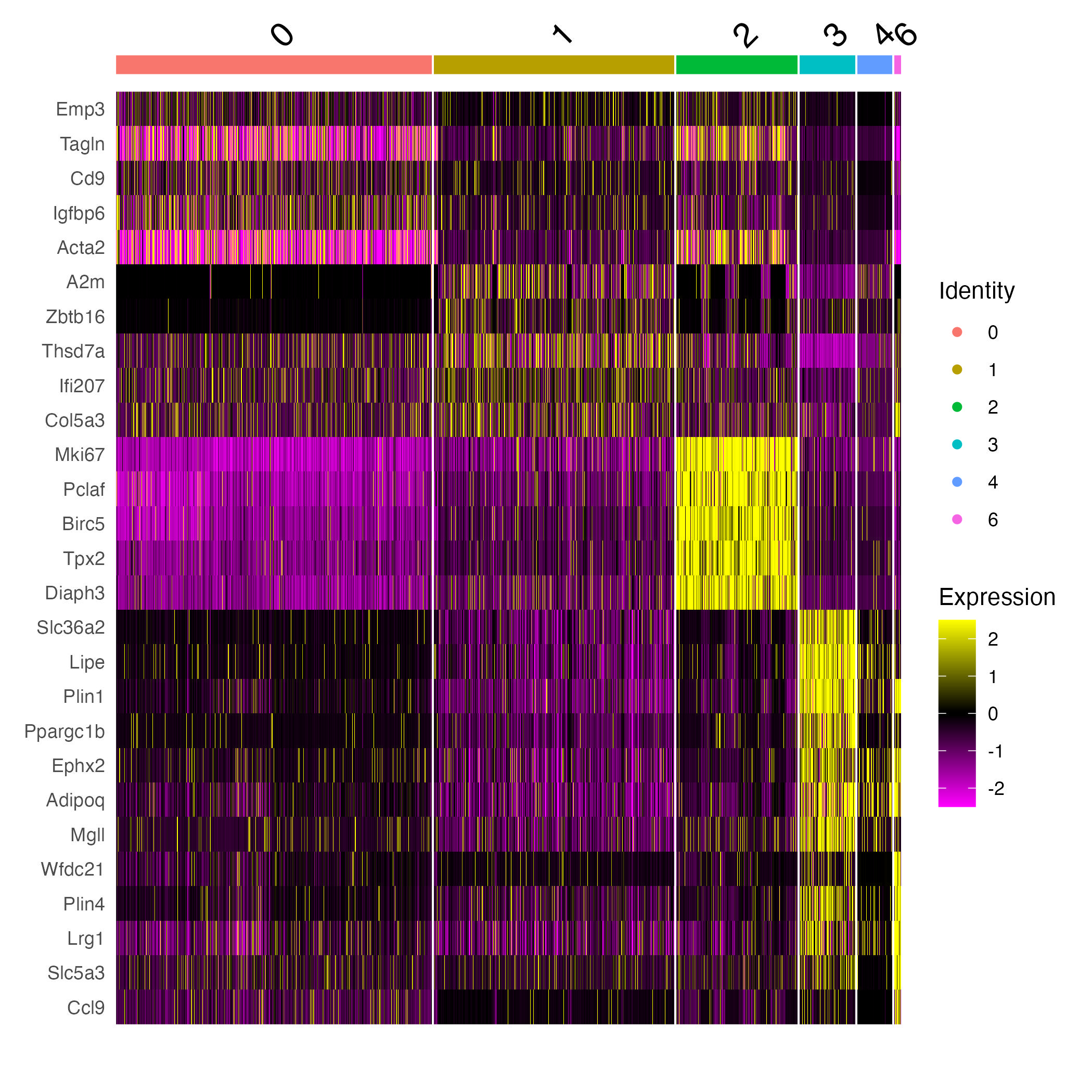
Finding markers between different time points (day 6 and day 0)

Idents(adp) = "time_point"
day6_day0_de=FindMarkers(adp,ident.1="Day 6",ident.2="Day 0",test.use="wilcox")
 

Visualizing clusters grouped by time points (day 6 and day 0)

fig1 = DimPlot(adp,group.by="time_point")
fig2 = FeaturePlot(adp,features="Acta2",order=T)
fig3 = FeaturePlot(adp,features="Cd36",order=T)
fig1/(fig2|fig3)
ggsave("dimplot_time_point.jpg")
 

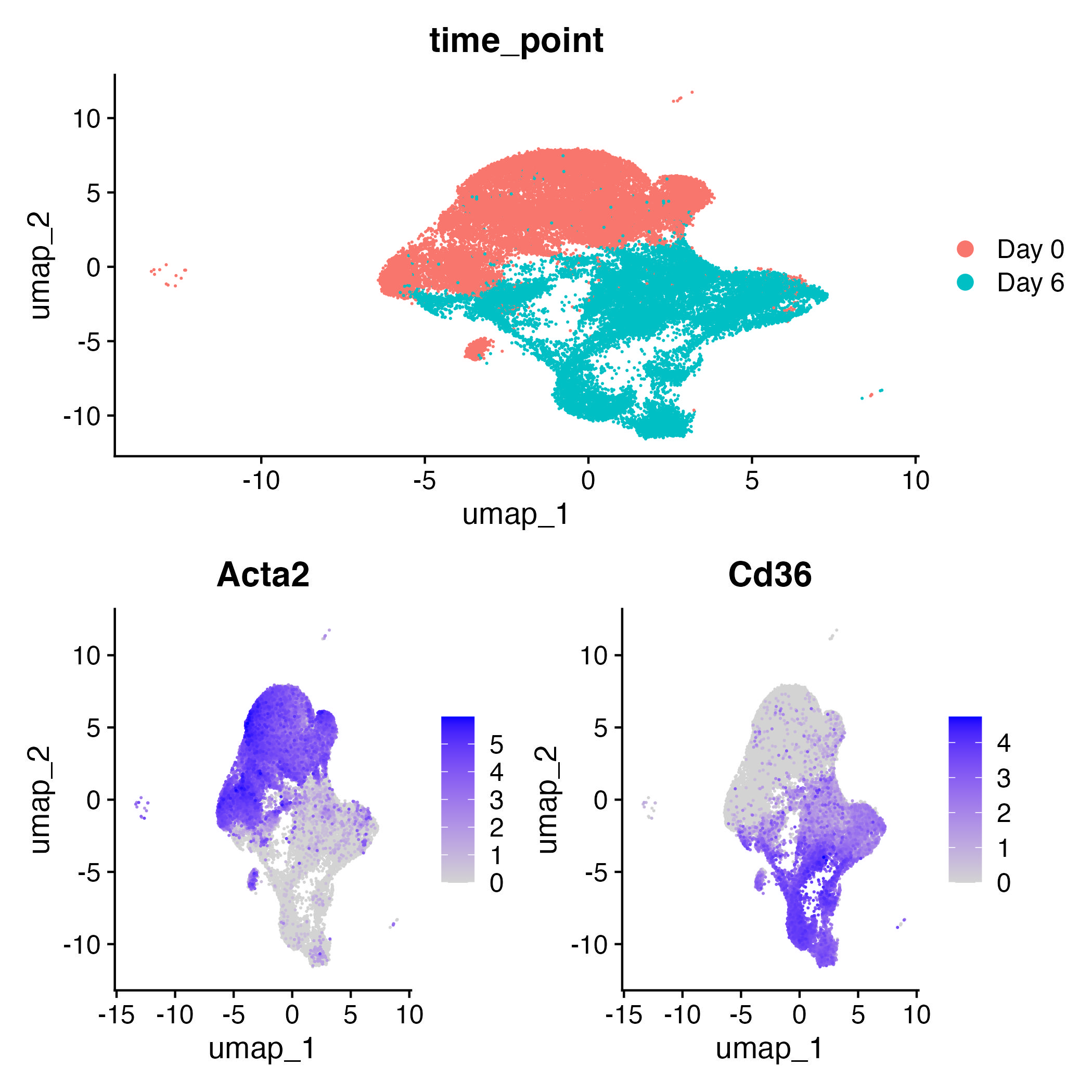
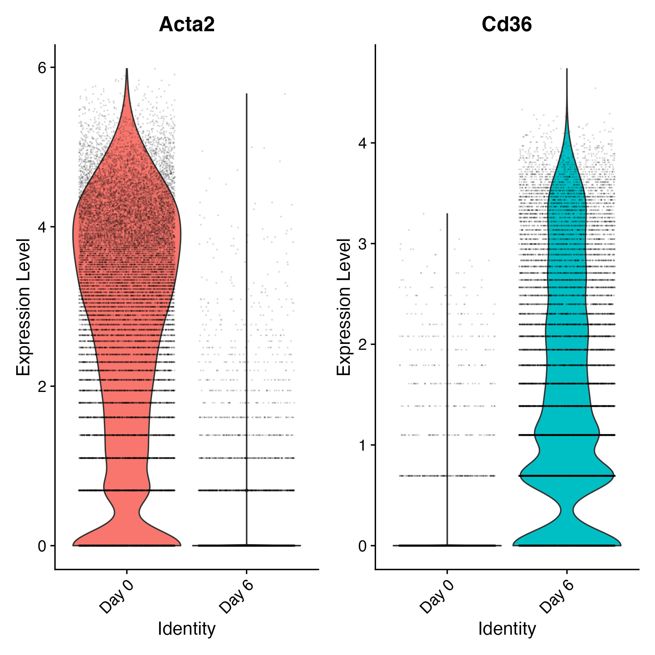
Acta2 is a marker of day 0, while cd36 is a marker of day 6.

Pseudobulk Differential Expression

The p-value inflation is a problematic point of scRNASeq analysis. The p-value inflation is a consequence of large sizes of compared samples. One approach to deal with the p-value inflation is to run a pseudobulk analysis.

Pseudobulk Differential Expression

pseudo_adp=AggregateExpression(adp,assays="RNA", return.seurat=T, group.by=c("orig.ident","time_point","condition","cond_tp"))
 

Cleaning metadata of the pseudo_adp seurat object

pseudo_adp = RenameCells(pseudo_adp,new.names=gsub("_.*","",pseudo_adp$orig.ident))
pseudo_adp$orig.ident=gsub("_.*","",pseudo_adp$orig.ident)
 

At this point, the count matrix of the pseudo_adp object can be feed into DESeq2 or edgeR for further analysis (pseudo_adp@assays$RNA$counts)

Finding DE markers between different time points of Pseudobulk analysis

Idents(pseudo_adp)="time_point"
bulk_adp_de = FindMarkers(pseudo_adp, ident.1="Day 6", ident.2="Day 0", test.use="DESeq2")
 

Comparing the results between the single cell and pseudobulk analysis

scDE.genes = rownames(day6_day0_de)[which(day6_day0_de$p_val_adj<0.05)]
bulkDE.genes = rownames(bulk_adp_de)[which(bulk_adp_de$p_val_adj<0.05)]
length(scDE.genes)
length(bulkDE.genes)
length(intersect(scDE.genes,bulkDE.genes))
 

11306
10516
8503
 

Significant overlap observed between single cell and pseudobalk analysis

Checking significance of DE expression in pseudobulk analysis for

bulk_adp_de[c("Acta2","Cd36"),]
 

                 p_val avg_log2FC pct.1 pct.2     p_val_adj
                                  
Acta2    1.256361e-274  -5.544797     1     1 3.129847e-270
Cd36      3.224132e-78   4.955947     1     1  8.031959e-74
 

Visuzlizing 5 top differentially expressed genes for each cluster in scRNAseq analysis

options(repr.plot.width=7, repr.plot.height=7)
Idents(adp)="SCT_snn_res.0.1"
DotPlot(adp,features=unique(top5$gene),dot.scale = 3)+coord_flip()
ggsave("dotplot_DE_genes.jpg")
 

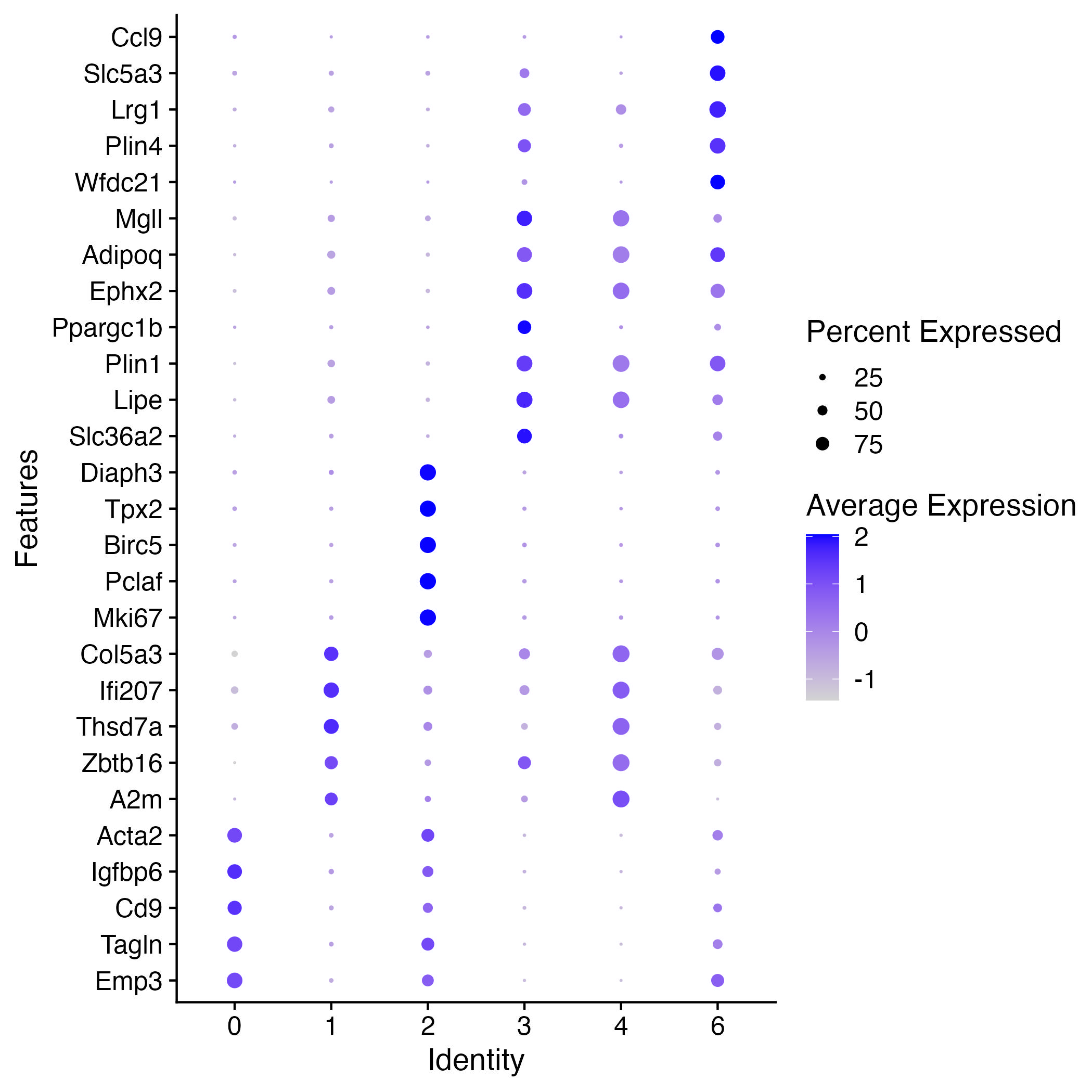
Another visualization of DE expressed genes is the violin plot

options(repr.plot.width=7, repr.plot.height=7)
Idents(adp) = "time_point"
VlnPlot(adp,features=c("Acta2","Cd36"),alpha = 0.1)
ggsave("violin_time_point.jpg")
 

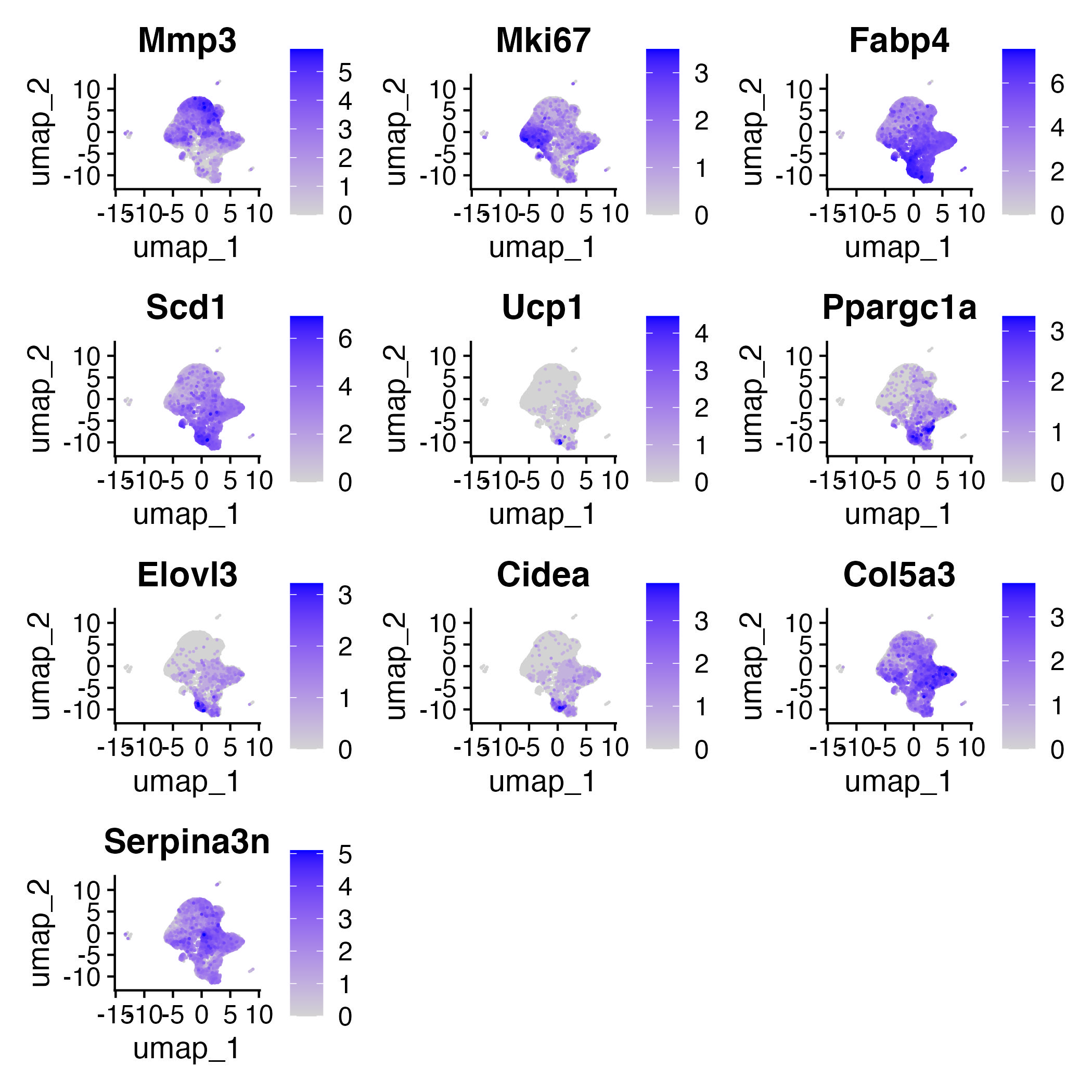
Cell anotation Annotation by DE Markers was obtained from the paper:
Mmp3: preadipocytes
Mki67: proliferating cells
Fabp4: differentiating beige adipocytes and differentiated beige adipocytes
Scd1: differentiated beige adipocytes
Ucp1: differentiated beige adipocytes
Ppargc1a: differentiated beige adipocytes
Elovl3: differentiated beige adipocytes
Cidea: differentiated beige adipocytes

br> Col5a3, Serpina3n: differentiating adypocytes

markers=c("Mmp3","Mki67","Fabp4","Scd1","Ucp1","Ppargc1a","Elovl3","Cidea", "Col5a3", "Serpina3n")
Idents(adp)="SCT_snn_res.0.1"
avgExp = AverageExpression(adp,markers,assay="SCT")$SCT
 

Cluster labeling

DimPlot(adp,label=T, label.size=6)
ggsave("dimplot_cluster_labels.jpg")
 

options(repr.plot.width=20, repr.plot.height=20)
FeaturePlot(adp,features=markers,ncol=3,order=T)
ggsave("Feature_plot_markers.jpg")
 

From the above graphs we can coclude:
Preadipocytes: Clusters 0 (Mp3)
Proliferating cells: Clusters 2, 6 (Mki67)
Differentiating beige adipocytes: Cluster 1
Differentiating adipocytes: Cluster 1, 4

Based on the above cluster assignments the final cluster labelling:

options(repr.plot.width=10, repr.plot.height=12)
adipocyte=vector(length=ncol(adp))
adipocyte[which(adp$SCT_snn_res.0.1 %in% c(0))]="Preadipocytes"
adipocyte[which(adp$SCT_snn_res.0.1 %in% c(2,6))]="Proliferating cells"
adipocyte[which(adp$SCT_snn_res.0.1 %in% c(1,4))]="Differentiating adipocytes"
adipocyte[which(adp$SCT_snn_res.0.1 %in% c(3))]="Differentiated beige adipocytes"
adp$adipocyte = adipocyte

f1 = DimPlot(adp,group.by="SCT_snn_res.0.1",label=T) + NoLegend()
f2 = DimPlot(adp,group.by="time_point") + NoLegend()
f3 = DimPlot(adp,group.by="adipocyte",label=T)+NoLegend()

(f1|f2)/f3
ggsave("final_labelling.jpg")
 

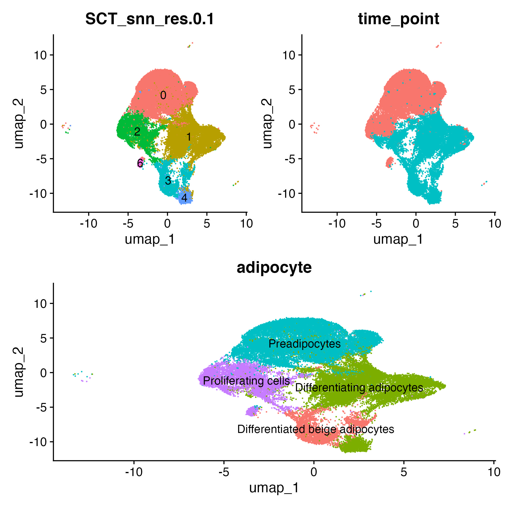
Conclusion: Preadipocytes and proliferating cells are mapped to day 0, while differentiated adipocytes, and differentiated beige adipocytes are mapped to day 6. There is a slight difference between the paper labeling and the current analysis labeling that can be attributed to the different reference transcriptome (2024 release year for the current analysis and 2020 release year in the paper analysis), cellranger and seurat versions.

Back to bioinformatics project page: Back to bioinformatics project page

Back to home: Back to home